Introduction
Since the internet boom a few years ago companies started to collect and save data in an almost aggressive way. But the huge amounts of data are actually useless if they are not used to gain new information with a higher value. I was always impressed by the way how easy statistical algorithms can be used to answer extremely complex questions if you add the component “Machine Learning”. Our goal was to create a web service that does exactly that thing: We realized Weather Forecasts using Machine Learning algorithms.
The Application can be split in four parts:
- The website is the final user interface to start a query and to see the resulting prediction.
- The server connects all parts and hosts the website.
- The database stores all important data about the weather.
- IBM Watson is used to calculate the forecasts with the data of the database.
In the following I will explain the structure more detailed and show how we developed the application.
Development
The Database
First, we needed the right data about the weather to start with. The idea was to connect our application with the weather API hosted at IBM Bluemix. Unfortunately, it did not work out because first the data we found there was useless for our aimed predictions and second the service was too expensive. So, what we did is, we took the free weather data provided by the DWD (Deutscher Wetter Dienst) and saved it at our own database hosted at Bluemix. The data includes all important information from 12/23/2015 until 6/20/2017 so only predictions in this range are logically possible and comparable to the actual values.
Machine Learning with IBM Watson
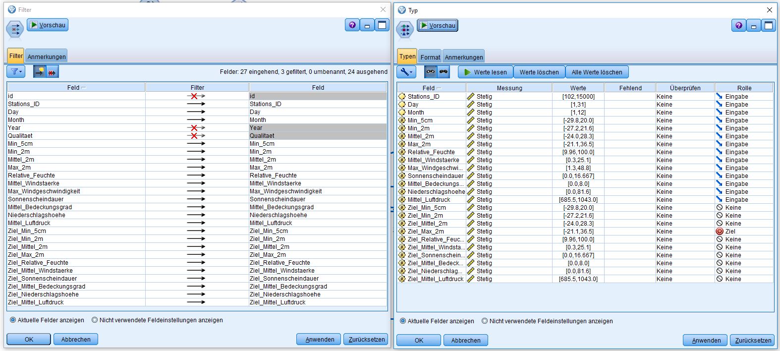
We created the prediction models with the SPSS Modeler by IBM. These so-called streams can be uploaded directly to the Watson Machine Learning Service. To create a stream based on our data, we first had to connect the database we used to train the model with the SPSS Modeler. The next step was to filter the data and to leave out all information that was irrelevant for creating the prediction model, for example the ID of each record as it has no influence on the predicted values. The records contained in the database are adapted to the model that predicts the weather for a chosen day using the information of one day before. This is why each record contains all measurements of one day and the measurements of the following one. Then all inputs and the relating outputs or results that will be predicted are marked at the field operation “type”. The measurements that were not used in this prediction model are marked with the role “none” to exclude them from the following computation.
On the following picture you can see the filter operation (left) and the type operation (right):
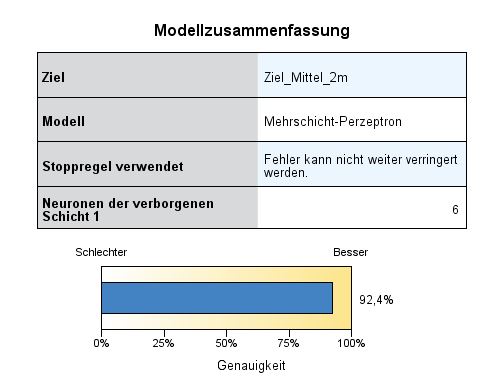
The Data was now ready for modelling and the auto numeric operation of the SPSS Modeler could calculate the models. The auto numeric operation calculates different kind of model types and chooses the one with the best results. For the prediction based on one previous day a neural network was defined to be the model with the best results.
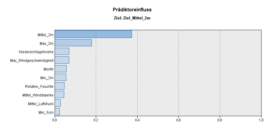
The figure below shows the features with their weights which represent the importance for the prediction. You can see that the middle and maximum temperature of the previous day have the biggest impact on the result.
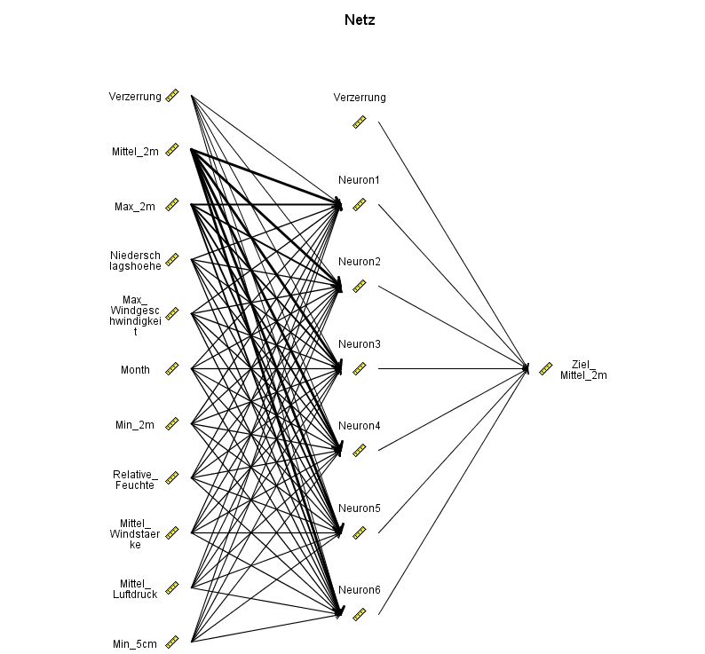
The calculated neural network has one hidden layer with six neurons and is shown below:
To produce the models which use two or four previous days to predict the next day, the datasets had to be adjusted within the SPSS Modeler. Every data set must contain the measurements of the two or four previous days as well as the data of the day for the prediction. For that we had to use operations for choosing, filtering, connecting and ordering data. In the following picture, you can see the stream which uses four previous days for calculating the model.
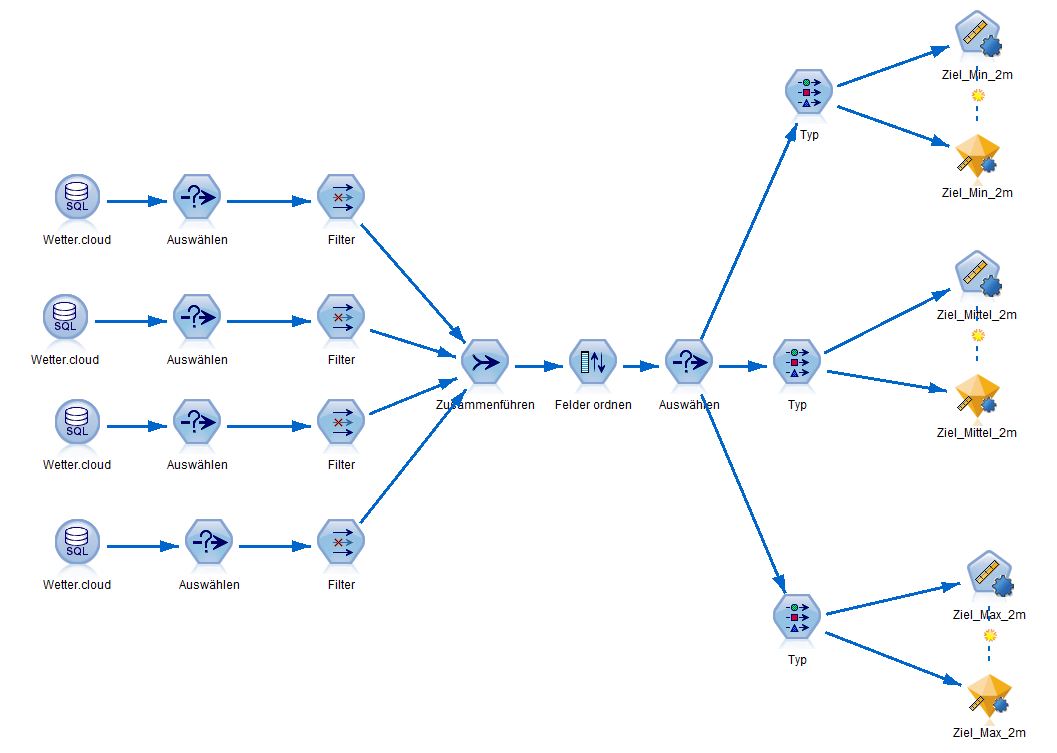
After executing the stream, a model is created (yellow diamond at the right site) that can be used in another stream which is used for calculating the resulting prediction and uploaded at Bluemix.
We noticed that including the data of two or four previous days as input at the prediction model instead of the data of only one day creates only minimal better results (1 day: 92,4%, 2 days: 92,9%, 4 days: 92,8%).
Server and website
After uploading the streams to Watson at Bluemix, we connected all parts with a Node.js server and created the website. As this was only a side aspect of the project, I would not describe this process more detailed.
The Result
You can test the web service at wettersave.mybluemix.net. You will see that only dates from 12/23/2015 until 6/20/2017 are possible to predict as described at the paragraph about the database.
If you are interested in the code, you can find it at the following GitLab repository:
https://gitlab.mi.hdm-stuttgart.de/sh245/cloud
Leave a Reply
You must be logged in to post a comment.