Don’t we all appreciate a little help in our everyday lives? “Alexa, turn on the lights in the living room.”
Voice assistants, smart lights and other smart home devices are all part of the Internet of Things (IoT). Those and other possible applications of IoT devices increase continuously and with it the overall number of connected devices. According to IoT Analytics Research, there are already over 12.3 billion connected IoT devices around the world, whereas most of them are wireless.
But how can we guarantee security, trust and liveliness in such networks?

Today, we will gain an insight into how byzantine fault tolerance can be achieved in wireless IoT networks. In particular, we will look at an analytical modeling framework by Onreti et al. for applying the Practical Byzantine Fault Tolerance (PBFT) algorithm to such networks. Furthermore, we will see which restrictions apply and how the viable area for these networks can be obtained. For more details, take a look at the original paper “On the Viable Area of Wireless Practical Byzantine Fault Tolerance (PBFT) Blockchain Networks” by Onreti et al. [2].
IoT and Blockchain
All devices (or nodes) in a fully autonomous IoT network communicate in a distributed way. However, this communication style is not an easy task as nodes need to agree on the validity of communicated data. The approach, for achieving the necessary level of security and trust, is to apply an appropriate consensus method. As the principle of agreeing on new data is the same as in blockchain, its consensus methods can also be applied to IoT networks. However, commonly used methods such as proof of work and proof of stake rely on computational power – a limited resource for most IoT devices. This is where wireless PBFT protocol comes in handy.
Practical Byzantine Fault Tolerance (PBFT)
Here, (wireless) PBFT refers to a blockchain consensus method with low computational complexity and power suited for asynchronous IoT environments.
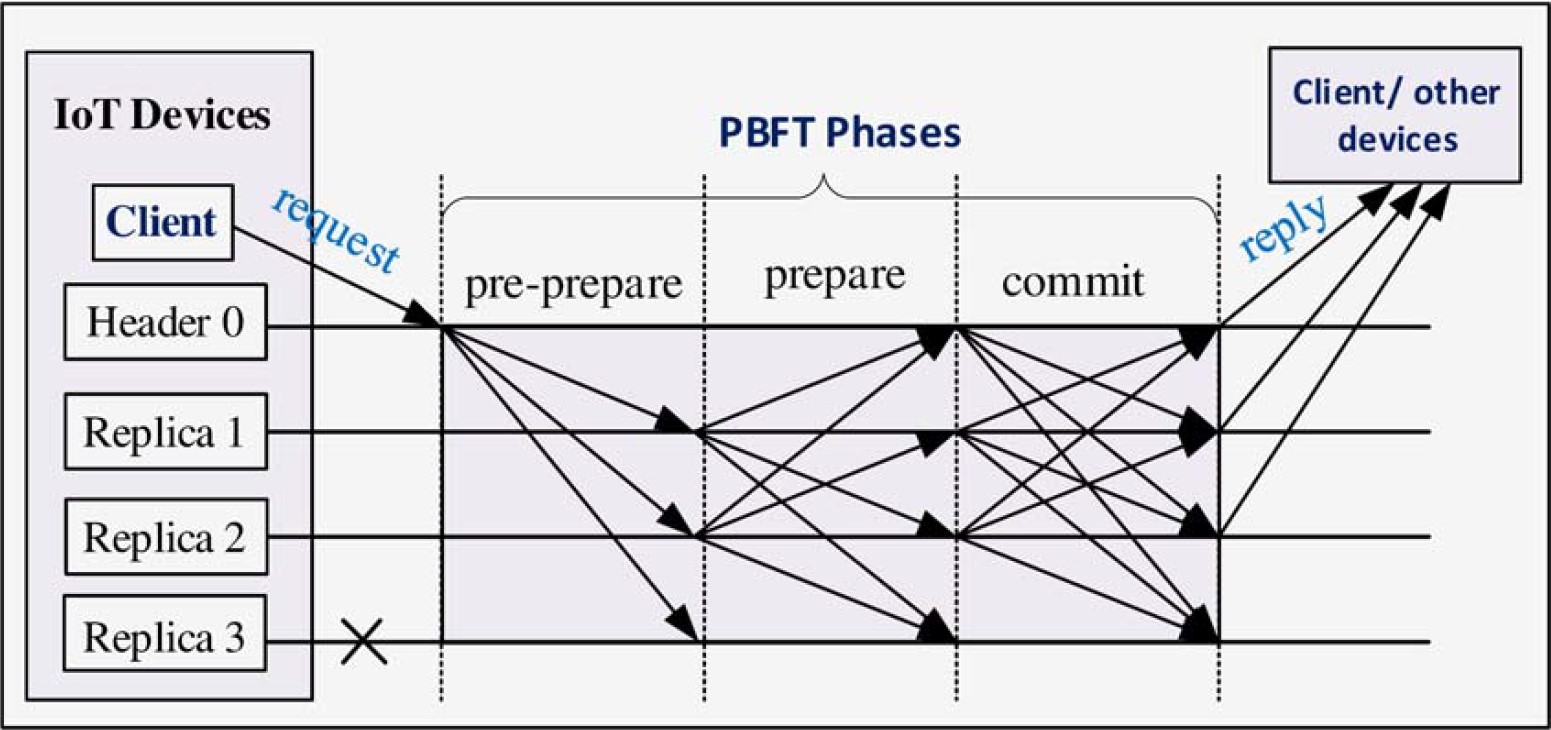
The protocol consists of the following three phases
- pre-prepare
- prepare
- commit
during which nodes communicate via wireless channels. Phase one is triggered as soon as a client node’s IoT request is received. The node receiving said request is referred to as header node, whereas all other nodes in the network are called replica nodes. In other words, a PBFT network is composed of several replicas and one leader, whereby the leader is reselected when it turns faulty or breaks down.
The protocol guarantees liveliness and safety as long as no more than (n-1)/3 of n replica nodes are faulty: f ≤ (n-1)/3.
The Protocol
The following steps describe the procedure from a request to a new block on the blockchain:
- request: A client device sends a request to the header node of the network.
- pre-prepare phase: The header node receives said request and broadcasts a pre-prepare message to the replica nodes.
- prepare phase: When a replica accepts a pre-prepare message, it enters the prepare stage. In this stage the replica broadcasts a prepare message to the network (including itself).
Before entering the next phase, a node needs to receive 2f prepare messages from different (but not necessarily other) nodes. In addition, those messages need to match the previous pre-prepare message. - commit phase: After receiving the necessary messages, a node will furthermore broadcast a commit message (including to itself).
Before leaving the commit phase, a node needs to receive 2f+1 matching commit messages from different nodes. Those 2f+1 messages usually contain a message from itself and the header. - reply: As soon as a node meets the previously mentioned condition, it will send a reply to the client.
- consensus & record: The client receives replies from the other nodes and proceeds as soon as the network reaches consensus in the form of f+1 matching reply messages. Lastly, the client records the transaction on the blockchain.
For more details of the original algorithm from 1999, take a look at “Practical byzantine fault tolerance” by M. Castro and B. Liskov [1].
Wireless PBFT: Assumptions & Restrictions
Onreti et al. [2] make the following assumptions about the PBFT network:
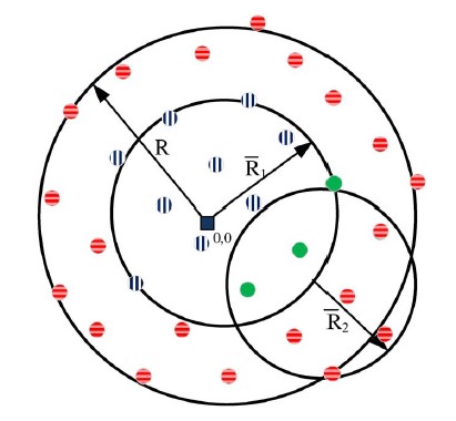
- Replica nodes are evenly distributed inside a circular area with radius R. Henceforth, λ denotes the density of n replicas inside this network area.
- The wireless network is noise limited: all replica nodes have equal receiver sensitivity, denoted by β1.
Based on the those assumptions, a header or replica node’s coverage radius Ri is defined by:
Ri = d0 [PiK/β1]1/γ ,
with:
- do: reference distance for antenna far field
- Pi: node’s transmit power
- β1: receiver sensitivity
- K: unit-less constant, dependent on antenna characteristics
- γ: pathloss exponent.
This formula highlights the main restrictions of the network’s nodes. Besides that, most IoT devices are further restricted by limited bandwidth and battery power. For this reason, the nodes’ workload should be kept as small as possible.
Based on the PBFT algorithm, there are further restrictions:
- The header node’s coverage area A1 needs to contain at least 3f+1 replicas:
A1λ ≥ 3f + 1 - For a non-faulty replica node, the coverage area A2 needs to overlap with the header node’s area A1. This intersection must contain at least 2f-1 other replica nodes:
A2λ ≥ 2f − 1 - Furthermore, a client’s coverage area A3 (while overlapping with A1), needs to contain at least f+1 replicas:
A3λ ≥ f + 1
The third constraint guarantees a successful reply to the client.
Constraints 1 and 2 guarantee the security and liveliness of the protocol and its three phases. Those constraints define the needed minimum of nodes for wireless PBFT. For a fixed number of faulty replicas f, additional nodes decrease the performance, as there are more messages (to be processed) as the protocol needs.
Viable Area
The viable area describes that (sub-)area of the network that fulfills all the constraints of wireless PBFT. This means, the number of nodes (and their placement in the area) need to be given such that:
- the header node can reach a minimum of 3f+1 replica nodes; where f denotes the number of faulty nodes
- a minimum number of matching messages (sent by different nodes) in the prepare (2f) and commit phase (2f+1) is achievable. This leads to:
Every single replica needs to be reachable by a minimum of 2f-1 other replicas. - a client node (located in- or outside of the network) can receive a minimum of f+1 matching replies
Furthermore, the concept of viable area is defined for a given view, which is determined by its specific header node. In other words, the view changes as soon as another node takes the turn in leading the network. A change of view happens at the latest when the current header fails or breaks down. Thereby the choice of header is well-defined by the view number v and the number of nodes n by i = v (mod n), where i denotes the index of the node in the network.
By determining the viable area, we can minimize the activation of nodes in the network. The smaller the nodes’ broadcast radius, the less nodes are activated. Thus, by minimizing the nodes’ coverage radius, we save energy and improve the performance.
All things considered, the viable area is dependent on:
- the number of replicas nodes n in the network
- the number of faulty replicas nodes f in the network
- the transmit power of header/replica nodes
- nodes’ receiver sensitivity
- pathloss components
(Mathematical) Approach for Determining the Viable Area
In order to find a minimum, the mathematical approach is to solve an objective function.
In this case, we are searching for the minimal coverage radius of the header and replica nodes. As the pathloss exponent γ and receiver sensitivity β1 can be considered fixed, this is the same as minimizing the nodes’ transmit powers Pi. Thus, the objective function is:
minimize P1 + P2
whereby P1 is the header’s transmit power and P2 is the transmit power of a typical replica node, that is at the very edge of the area.
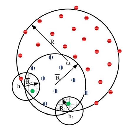
Based on the header’s placement, and therefore the shape of the areas A1 and A2, the terms describing the protocol’s first two constraints differ. There are two different cases as depicted below:
![]() ,
,![]() ,
,![]() : all nodes of the network (area)
: all nodes of the network (area)
![]() ,
,![]() : nodes inside header node’s coverage area
: nodes inside header node’s coverage area
![]() : nodes inside replica node’s coverage area
: nodes inside replica node’s coverage area
In case 1, the header is located at (or near) the origin and has a circular coverage area A1 dependent on its coverage radius. In the second case, A1 is no longer circular but rather an intersection of two circular areas; i.e. A1 is additionally dependent on the header’s distance to the origin and the radius R of the network. In this case, the reference “replica on the edge” for the second constraint is located at an intersection point (h1 or h2), which represents the minimal possible A2.
In both cases, we adjust the coverage radiuses Ri (respectively the transmit power Pi) such that the areas fulfill the first two constraints of the protocol.
Solving for Pi
So far, we have an objective function with two constraints. In order to find reasonable results, we furthermore restrict the searched parameters:
In this case this means that the transmit powers Pi need to be limited. We set the header node maximum transmit power P1max, such that the header can still reach every node in the network, if needed. Furthermore, we set the maximum of P2 such that P2max = αP1max , with α > 1, i.e. P2max is greater than P1max.
As a consequence, we restrict P1 and P2 by:
0 ≤ P1 ≤ P1max
0 ≤ P2 ≤ P2max
With this additional constraint, we can solve the objective function using a classic method and denote its result as P1* and P2*.
Up to this point, the third constraint for wireless PBFT has been ignored. This constraint focuses on the last step in the protocol: the reply to the client. Thus, we need a coverage area A3 (dependent on the given P1*), such that at least f+1 replicas can reach the client. Based on the client’s receiver sensitivity β2 and its distance to the header node, we can use a linear search method for determining the transmit power Pc of a replica needed for replying to the client.
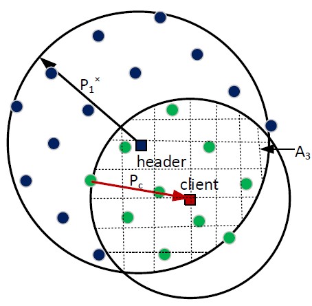
by the replicas when responding to the client (IoT device). [2]
Numerical Results
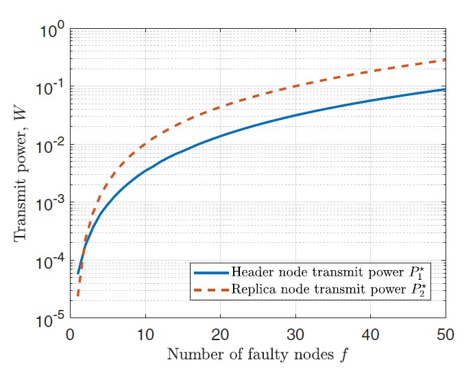
λ = 1/(π1000) nodes/m2. [2]
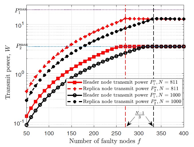
λ = N/(π10002) nodes/m2, N = 811, 1000. [2]
The previous diagrams show the transmit powers of header and replica nodes in relation to the number of faulty nodes. The values have been determined for a view with the header at the origin. Further system parameters for these results can be found in [2].
Both diagrams show that the transmit power of header and replica nodes increases with the number of faulty nodes. That is because their coverage areas need to include more nodes.
Furthermore, the right diagram shows two more important points. First, a higher node density reduces the needed transmit power. Second, we can see the restrictions of the transmit power: it is not only restricted by (n-1)/3, but also by the maximal transmit power P1max resp. P2max.
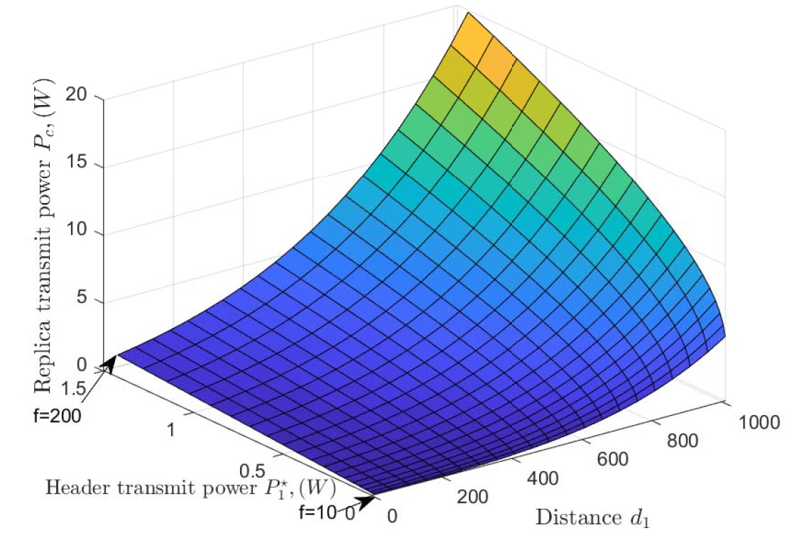
power during the reply phase, λ = 1/(π1000) nodes/m2. [2]
Last but not least, the diagram to the left shows the increase of transmit powers with increasing number of faulty nodes f. As expected, the needed replica’s transmit power Pc increases with the distance d1 of the client to the header; but in particular, we can also see that it really ramps up with an increase in faulty nodes f.
Critique: Advantages and Drawbacks of Wireless PBFT
Applying PBFT to IoT blockchain networks has clearly benefits over other methods, as it needs less resources. But how applicable is this approach to an existing network? It seems rather questionable, whether an existing network can fulfill the required assumptions. When the nodes are not evenly distributed, this approach for determining the viable area can not be applied. Furthermore, the needed noise limitation might not be given. However, when the assumptions are met, the constraints for A1 and A2 of the viable area can also be used to check whether a transaction is indeed successful [2].
The last point seems rather important. If anything in the network changes, it probably has an impact on the viable area and thus on the needed transmit powers. The PBFT algorithm has some mechanism in place to change the view, if needed – but Onreti et al. do not address what exactly happens when nodes crash or have exhausted their battery.
Besides verifying successful transactions, constraints 1 and 2 of the viable area can be used in the design for a new network – in particular for determining the radius R. [2] We might say we have a trade-off between energy savings (per node) and the overall number of nodes for a network. When we add additional nodes – to an otherwise similar network – we increase the node density. If the number of faulty nodes stays the same, this leads to energy savings. However, there is no guarantee that the rate of faulty nodes does not increase with the number of overall devices; and even though a higher node density decreases the needed transmit power, additional nodes bring other costs with them (e.g. maintaining the network).
Open Questions
Some questions persist: Who keeps track of the number of nodes n? Can the number of nodes change? When nodes turn off due to an exhausted battery, do we just consider them faulty or remove them (i.e. n reduces and node’s indices change)? Removing nodes from the network, would at least mess with the assumed node distribution. For that reason, it seems likely that we just consider exhausted nodes faulty. That brings us to the next question: Who keeps track of the number of faulty nodes? How big is the resource consumption for determining the number of faulty nodes? Who calculates the minimal transmit powers and how often are they recalculated? And what happens if the noise increases?
I would like to see a direct comparison of the power consumption of a test PBFT network, with the same network using another consensus method. Furthermore, numerical results for the case of a header at the edge of the network (worst case of case 2) would be interesting; as well as some sort of ratio of possible views in a network in relation to the header placement (i.e. case 1: case 2).
Last words
Actually, researchers have done a fair amount of work surrounding pBFT/PBFT in the past 2 years, further optimizing the original consensus method. Some of the work, namely SHBFT [3] and G-PBFT [4], (even though not specifically focusing on wireless) also address blockchain IoT networks explicitly. Even though PBFT has already been elaborately examined in 1999, the current research further emphasizes that byzantine fault tolerance is still not that easy to achieve.
On a final note I would like to say: Consensus methods often have such easy rules – in theory – as long as you don’t have to implement them.
Sources
[1] M. Castro and B. Liskov, “Practical byzantine fault tolerance”, Third Symposium on Operating Systems Design and Implementation, New Orleans, USA, Feb. 1999
[2] https://ieeexplore.ieee.org/abstract/document/9013778
O. Onireti, L. Zhang and M. A. Imran, “On the Viable Area of Wireless Practical Byzantine Fault Tolerance (PBFT) Blockchain Networks,” 2019 IEEE Global Communications Conference (GLOBECOM), pp. 1-6, doi: 10.1109/GLOBECOM38437.2019.9013778, 2019
[3] https://doi.org/10.1007/s12083-021-01103-8
Li, Y., Qiao, L. & Lv, Z. “An Optimized Byzantine Fault Tolerance Algorithm for Consortium Blockchain”, Peer-to-Peer Netw. Appl. 14, 2826–2839, 2021 https://doi.org/10.1007/s12083-021-01103-8
[4] Lao L, Dai X, Xiao B, Guo S,” G-PBFT: a location-based and scalable consensus protocol for IOT-Blockchain applications”, 2020 IEEE International parallel and distributed processing symposium (IPDPS). IEEE, pp 664–673, 2020
Leave a Reply
You must be logged in to post a comment.