Google’s Spanner

A Question of Time and Causality

TL;DR

Through the usage of atomic clock and GPS in datacenters, Google is able to determine a worst-case clock drift that may develop between set intervals, after which the normal quartz clocks of the machines will be synced with the atomic clock. By already having a very good estimate of the actual physical time and knowing the worst-case drift, an interval will be delivered to planned transactions, that are ready to be committed. Once received, the transaction will wait for the duration of the interval and thus ensuring causal consistency of a following transaction will be fulfilled. The key to solving this issue turns out to be atomic clocks, GPS receivers, testing to determine the uncertainty interval and a regular synchronisation of all sub-systems, not directly connected to their True Time service.

What is Google’s Spanner?

Google Spanner [B017] is a relational database service provided by Google Cloud, designed for processing and storing petabytes of structured data. Spanner provides global distribution of data with high consistency and availability, as well as horizontal scalability. According to the CAP theorem [GL02], Spanner is therefore a CA system. It supports SQL-like query languages as well as ACID [C970] transactions (Atomicity, Consistency, Isolation, Durability) and is capable of providing both horizontal and vertical scalability to achieve better performance.

This is an answer that one can formulate after a few minutes of using the Google search engine. But what defines the service? What unique features make Google’s Spanner stand out and how are they technically formulated and implemented? This will be conveyed in the course of this blog post.

What defines Google’s Spanner?

To make our lives easier while explaining and understanding what actually defines Spanner, the significant descriptive characteristics of Spanner are separated into two sections: Consistency properties and techniques used to realise them.

Properties of Consistency:

Serializability writes

In transactional systems, there exists an execution plan for parallel execution. This plan is called history and indicates the order in which the different operations of the transaction shall be executed. Such a history will be serializable, if and only if it will lead to the same result as the sequentially executed sequence of the history’s transactions.

Linearizability reads and writes

This is a concept in database systems that ensures that the execution of concurrent operations on a shared object or resource appears as if they occurred in some sequential order. This means that even though operations are being executed concurrently, they appear to be executed one after the other.

Serializability vs Linearizability

Did those two sound too similar? They are not! Subtle details make a big difference here: Even if both serializability and linearizability are concepts related to concurrency control in database systems, they have different goals and focus on different aspects of concurrency. While serializability ensures that concurrent transactions produce the same result as if executed sequentially, maintaining data integrity and equivalent results to executing transactions sequentially; Linearizability ensures that concurrent operations on a shared object or resource appear to be executed sequentially, maintaining data consistency and equivalent outcomes to executing operations sequentially.

Techniques in use:

Sharding

Spanner supports a custom sharding algorithm called “Zone Sharding.” [AR18]. This algorithm partitions data across zones, which are groups of machines in a single datacenter or across multiple datacenters. Each zone contains multiple tablet servers that hold the data for a subset of the database’s tables. The Zone Sharding algorithm is designed to ensure that data is replicated and distributed for high availability and fault tolerance, while also providing efficient access to data with low latency. Especially the low latency is of tremendous importance, for many of the services of Google.

State machine replication (Paxos protocol)

The Paxos protocol [L998] is a consensus algorithm that helps distributed systems agree on a single value despite failures or network delays. First it was described by Leslie Lamport in 1989 and has since become widely used in distributed computing systems. It operates in three main phases:

Prepare Phase: A proposer suggests a value to the other nodes and asks them to promises not to accept any other value in the future.
Accept Phase: If the majority of nodes promise to accept the proposed value, the proposer sends an “accept” message to all the nodes, including the proposed value.
Commit Phase: If the majority of nodes accept the proposed value, the proposer sends a “commit” message to all the nodes, indicating that the proposed value has been agreed upon.

The Paxos protocol has been used in a variety of distributed systems, including databases, file systems, and messaging systems. It is known for its simplicity, generality, and ability to tolerate failures. However, it can be complex to implement and can suffer from performance issues in certain scenarios.

Two-Phase locking for Serializability

Two-phase locking (2PL) [G981] is a concurrency control mechanism used in database management systems to ensure serializability of transactions. The goal of 2PL is to prevent conflicts between transactions by ensuring that a transaction holds all necessary locks before performing any updates.

The two-phase locking protocol operates in two main phases:

Growing Phase: During this phase, a transaction can acquire locks on database objects (such as rows, tables, or pages) in any order. However, once a lock is released, it cannot be re-acquired.
Shrinking Phase: During this phase, a transaction can release locks but cannot acquire any new ones. Again, once a lock is released, it cannot be re-acquired.

The 2PL protocol ensures serializability by guaranteeing that conflicting transactions acquire locks in a consistent order. Specifically, two transactions conflict if they access the same database object and at least one of them performs an update.

Two-Phase Commit for cross-shard atomicity
The Two-Phase Commit (2PC) [H983] is a distributed algorithm used to ensure atomicity in transactions that involve multiple nodes or resources. The protocol works in two main phases:

Prepare Phase: In this phase, the transaction coordinator asks each participant to vote on whether to commit or abort the transaction.
Commit Phase: If all participants vote to commit, the coordinator instructs each participant to commit the transaction. If any participant votes to abort, the coordinator instructs each participant to abort the transaction.

2PC ensures that a transaction is either committed or aborted atomically across all participants involved in the transaction, but can suffer from performance issues and a higher risk of aborts. Alternative protocols, such as optimistic concurrency control or decentralised commit protocols, can be used to address some of these issues.

Multi-Version Concurrency Control

Multi-Version Concurrency Control (MVCC) [B981] is a database concurrency control mechanism that allows multiple transactions to access the same objects simultaneously while maintaining consistency and isolation. It creates multiple versions of a database object and allows each transaction to access the version that corresponds to its snapshot of the database. MVCC provides benefits such as reduced lock contention, improved scalability, and higher degree of concurrency and isolation, and is used in various database systems like PostgreSQL [PSQL] or MySQL [MSQL]

Now, how does MVCC actually work? Short answer, with strong implications: A timestamp $t_w$ is being attached to every read-write transaction taking place. If a transaction is going to change an object, we will not simply allow it to change its state, but rather make a copy of the object, change the copy and tag it with the timestamp of the transaction $t_w$ . This is to ensure, that if a read-only transaction comes in, interested in the old state of the object (with a timestamp $t_{w-1}$ ), we still can serve it. Now, a new read-only transaction $T_r$ comes in, tagged with $t_r$ where $T_r > T_w$ . This transaction can simply ignore all states of objects where $t_w > t_r$ and pick those with the most recent state $t_w \leq t_r$ .

So far, even if implementing the above correctly would bring quite an engineering challenge to the table, there is nothing new or innovative. Nothing special that is required to be mentioned, other than framing and explaining the used technologies. Spanner provides support for read-only transactions without the need for locks, a feature not found in other database systems – at least if MVCC is not implemented. This is a significant improvement over 2PL, which requires objects to be locked before access. However, in the real world, large read-only transactions are common. Take the example of a database backup, which is a major read-only transaction that can span multiple petabytes in a globally-distributed database. It is clear that users would not be happy about waiting for such a process to succeed. Imagine it fails and has to restart shortly after. A horrible scenario for every impatient user, if locks may be taken during that process. Spanner’s support for lock-free read-only transactions ensures that such processes can be carried out quickly and efficiently, enhancing user satisfaction and improving the overall performance of the system.
But, the really interesting part about Spanner is how it acquires said timestamps.

Consistent Snapshots

First, let us establish what it means to have a consistent snapshot. To illustrate this, we can use the example of a large read-only transaction, for example a backup, and clarify the requirements for ensuring snapshot consistency

What does it mean for a snapshot to be consistent?

A read-only transaction will observe a consistent snapshot if: $T_1 \rightarrow T_2$ . This means that if a consistent snapshot contains the effect of transaction $T_2$ , it must contain the cause $T_1$ . So if $T_1$ happened before $T_2$ and we have a snapshot that contains the writes by $T_2$ , it must also contain the writes mades by $T_1$ . Likewise, if we see a snapshot that does not contain the writes made by $T_2$ , is shall not contain the writes made by $T_1$ . In other words, snapshots must be consistent with causality – hence the title of this blog.

The above will be achieved by making use of MVCC.

True Time

Why do we need true time for a service like Google’s Spanner?

As any being interested in this subject matter will tell you: There is no free lunch in ultra large scale systems; most certainly, there cannot be a thing like a true time. Or maybe…

In the paragraph explaining what it means for a snapshot to be consistent, we clarified that we need to take measures to ensure a reliant way of dealing with the problem of chronological ordering, namely causality. Even though logical clocks like Lamport Clocks where specifically designed to address this problem, there are scenarios in which they would fail. Imagine a case in which a user would read a result from replica $A$ , perform an action on that data and may persist it on replica $B$ . A one-sentence scenario, in which Lamport Clocks would fail to solve the problem, simply because there was no assured communication between the two replicas. Sure, we could rely on the front-end developer to transport the timestamp for the write transaction on replica $B$ , but this is not guaranteed. Neither can we rely on the user to manually type in a timestamp. So, what can we do in this case: We go back to physical clocks. But, we have to adjust the physical clocks and do some extra measure, to ensure that causality is satisfied.

I’m on the hook, pull me in!

The way spanner achieves this, is by using its service called True Time. True Time [B017] is a system of physical clocks, that explicitly captures the always present uncertainty within the resulting timestamps and communicates it to the requestor. To help understand the impact achieved, we will use the following illustration as an example.

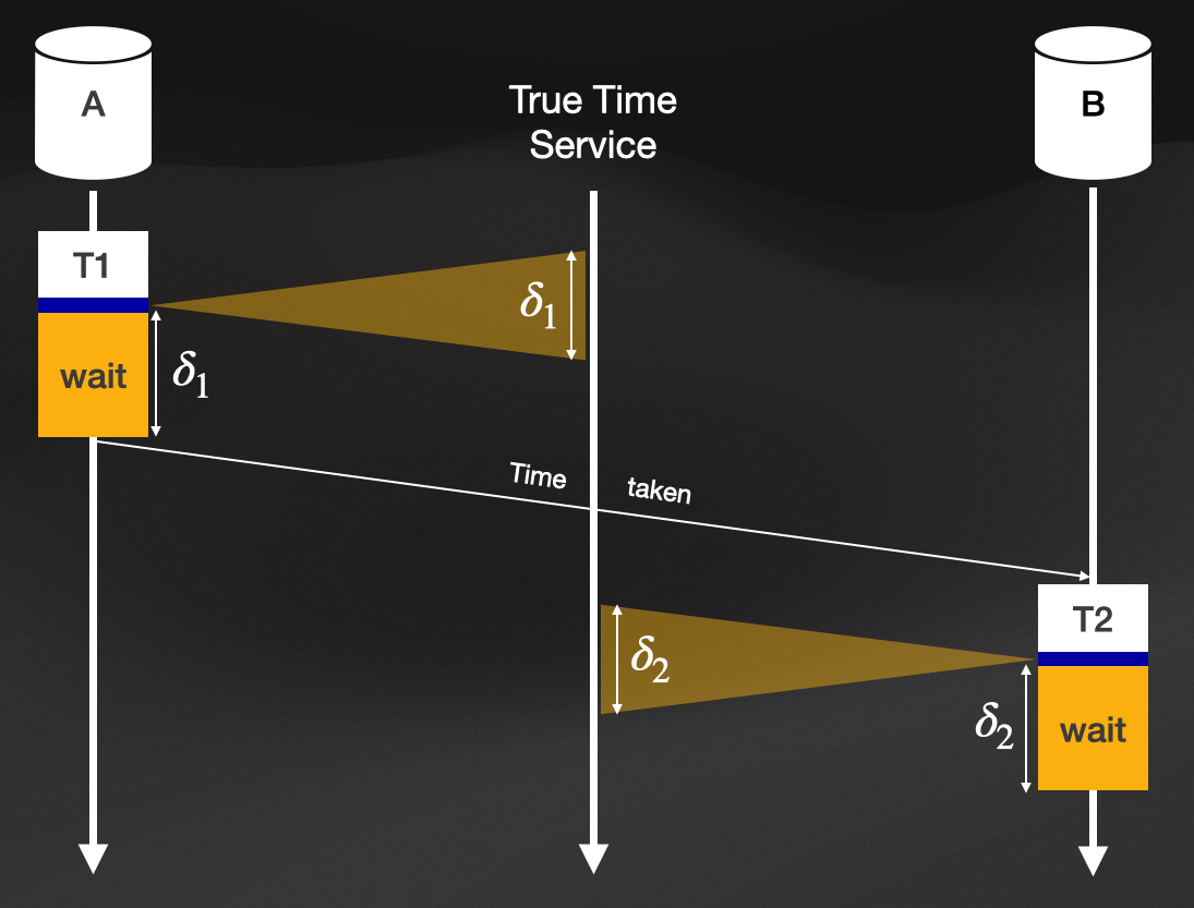
Graph showing the aggregation and exploitation of planned waiting intervals from True Time

In this illustration, we have two replicas: $A$ and $B$ . A write transaction $T_1$ will be performed on replica $A$ and a follow-up transaction $T_2$ will be performed on replica $B$ . Here, we have that physical time dependency between the two, such that their timestamps fulfil $t_1 < t_2$ .

When $T_1$ is ready to be committed, it requests the interval $\delta_1$ from the True Time Service. So, we do not just get a timestamp, as it is required for MVCC. Rather the requestor will receive two: $[t_{1min}, t_{1max}]$ . The first one $t_{1min}$ indicating the earliest possible and the second $t_{1max}$ indicating the latest possible actual time for the commit request to actually happen. Since there can not be a perfect synchronisation between the different clocks, within a datacenter, we can never be totally certain that a timestamp would represent the actual physical time of that moment. By accepting this fact and using an uncertainty bound through the received interval, we can ensure that the physical time would lie somewhere within that closed interval.

Spanners system is now delaying the transactions commit for the duration of the interval $\delta_1$ . During that wait-time, the system will continue to hold all the locks mandatory and be ready to release them. Once interval $\delta_1$ is elapsed, the transaction will actually be committed. This extra wait is the key concept here.

Now let us say that replica $B$ receives transaction $T_2$ and starts executing it. Similar to the procedure of $T_1$ , once $T_2$ is ready to be committed, it requests its pair of earliest and latest possible time $\delta_2$ , waits for the $\delta$ -time to elapse and commits its transaction. Remember, we have the physical time dependency $t_1 < t_2$ . The white arrow in the illustration, going from left to right, indicates the actual time elapsed between the end of $T_1$ and the start of $T_2$ .

What we just achieve ensures that the uncertainty intervals we receive from the True Time Service are warranted to be non-overlapping ant thus ensures that the causal dependency will be reflected. After the wait-time, MVCC will receive the maximum timestamp from $\delta_1$ and $\delta_2$ and the database only contains the effect, when its cause is present.

How uncertain do we have to be?

Of course, we want to have as little waiting-time as possible. This forces us to have a pretty precise notion of uncertainty. This is achieved by atomic clock servers, with GPS receivers in every datacenter. Even tough maintaining both probably costs quite some money, it is cheaper than dealing with potential inconsistencies in their system.

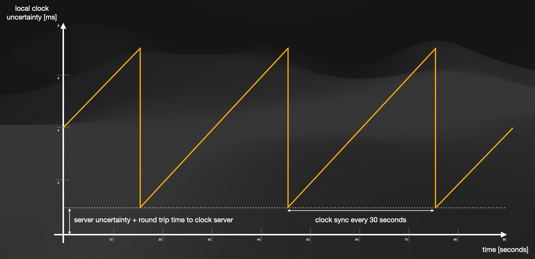
Illustration showing the clock drift of machines not directly connected to the True Time service

As the illustration shows, machines not directly connected to the True Time service will continue to drift apart form the physical time and continue to do so, until the clock synchronisation happens. After that, the discrepancy is immediately reduced to the irreducible error $E < 1ms$ , resulting from the time the request takes from a machine to True Time and back. During the 30-second intervals between periodic clock synchronisations, a node’s local quartz oscillator determines its clock. The error introduced during this period is influenced by the drift rate of the quartz. To err on the side of caution, Google assumes a maximum drift rate of 200ppm, which is much higher than the drift rate observed under typical operating conditions. Furthermore, Google keeps track of each node’s drift and informs administrators of any unusual occurrences.

Summary

True Time utilises precise accounting of uncertainty to establish both upper and lower bounds on the current physical time. It achieves this by incorporating high-precision clocks, which work to reduce the size of the uncertainty interval. Meanwhile, Spanner is designed to ensure that timestamps remain consistent with causality by waiting out any lingering uncertainty. By leveraging these timestamps for MVCC, Spanner is able to deliver serializable transactions without necessitating locks for read-only transactions. This method helps maintain transaction speed while also eliminating the need for clients to propagate logical timestamps.

References

GL02
S. Gilbert, N. Lynch; 2002
Brewer’s Conjecture and the Feasibility of Consistent, Available, Partition-Tolerant Web Services
https://www.comp.nus.edu.sg/~gilbert/pubs/BrewersConjecture-SigAct.pdf
C970
E. F. Codd; 1970
A Relational Model of Data for Large Shared Data Banks
seas.upenn.edu/~zives/03f/cis550/codd.pdf
CD12
James C. Corbett, Jeffrey Dean, Michael Epstein, Andrew Fikes, Christopher Frost, JJ Furman, Sanjay Ghemawat, Andrey Gubarev, Christopher Heiser, Peter Hochschild, Wilson Hsieh, Sebastian Kanthak, Eugene Kogan, Hongyi Li, Alexander Lloyd, Sergey Melnik, David Mwaura, David Nagle, Sean Quinlan, Rajesh Rao, Lindsay Rolig, Yasushi Saito, Michal Szymaniak, Christopher Taylor, Ruth Wang, Dale Woodford; 2012
https://static.googleusercontent.com/media/research.google.com/de//archive/spanner-osdi2012.pdf
AR18
Muthukaruppan Annamalai, Kaushik Ravichandran, Harish Srinivas, Igor Zinkovsky, Luning Pan, Tony Savor, and David Nagle, Facebook; Michael Stumm, University of Toronto; 2018
https://www.usenix.org/system/files/osdi18-annamalai.pdf
L998
Leslie Lamport; 1998
https://dl.acm.org/doi/pdf/10.1145/279227.279229
G981
Jim Gray, Paul McJones, Mike Blasgen, Bruce Lindsay, Raymond Lorie, Tom Price, Franco Putzolu, Irving Traiger; 1981
https://dl.acm.org/doi/pdf/10.1145/356842.356847
H983
Theo Haerder, Andreas Reuter; 1983
https://cs-people.bu.edu/mathan/reading-groups/papers-classics/recovery.pdf
B981
Phillip A. Bernstein, Nathan Goodman; 1981
https://dl.acm.org/doi/pdf/10.1145/356842.356846
PSQL
https://www.postgresql.org/docs/7.1/mvcc.html
MSQL
https://dev.mysql.com/doc/refman/8.0/en/innodb-multi-versioning.html
B017
Eric Brewer; 2017
https://storage.googleapis.com/pub-tools-public-publication-data/pdf/45855.pdf