Written by Marvin Blessing, Michael Partes, Frederik Omlor, Nikolai Thees, Jan Tille, Simon Janik, Daniel Heinemann – for System Engineering And Management
Introduction
The aim of the project was to develop a system with which the power consumption of any socket in a household is determined and stored in real time and can be read out by users with the corresponding access data. The user of the system should be able to read out the data via a web application to which he can log in with an account. This should also ensure mobile access to the data. Furthermore, the measured data should be permanently stored in a database, so that users also have the option of viewing measured values over a longer period of time.
The measurement of power consumption should be made possible with a hardware element that is attached to the socket and writes the measured values to the database described.

Fig. 1: Basic system structure
The finished system includes a hardware element and forwards the measured current to a database via a message broker. In addition, the system includes a front-end (web page) through which a user can then query this data via an individual user account.
A more detailed description of the architecture can be found in the following chapter “Architecture”.
According to statista.com there were about 3.6 million homes in Germany that used energy management applications in 2020. For the year 2025 there is an estimate of about 15.3 million homes using energy management systems. Therefore, taking competition and market growth into account, it’s not unlikely that a system like the one we created could reach 2 million homes in the near future.
Architecture
For the architecture of the project, we have to take a look at the system requirements which we defined based on the use case:
- Read power data
- Send power data from user to our system
- Store power data
- Store user data
- Read power data based on the user
- Visualize data for users
- Monitoring and logging
- (Authentification)
To implement these requirements, it is crucial to understand the needs of each requirement and figure out an efficient way to connect all the necessary components.
In the first step, we made a list of the technologies that we needed to implement those components:
- Read power data: To measure the power data we need a Raspberry Pi that has access to the sockets of the user. On the Raspberry Pi is a Python script running that collects the power data.
- Sending data from Raspberry Pi: To send the power data from the Raspberry Pi to our main system, we decided to use a message broker, since we have to be able to send a lot of data from many different users to our system at the same time.
- Store power data: To store the power data we use a simple timeseries Database because all data points have a timestamp.
- Store user data: For the user authentication we use a separate Database to store the user data.
- Read power data based on the user: To access the stored data we decided to use multiple small services which are used to perform tasks on the databases. This includes an user authentication service which checks the correctness of the provided user data, as well as a read service and a write service to access the stored power data and write new power data to the timeseries database.
- Visualize data for users: To visualize the data for the user we use a simple web app that uses the different services to access and present the power data to the user.
- Monitoring and logging: To check the status of our system we use some self defined metrics that we can observe through dashboards.
- (Authentification: We want to authenticate the user securely and therefore have planned an authentication service with Keycloak. However, this is not implemented at the current time.)
The connection of these components is shown in the following architecture diagram.

Fig. 2: The general architecture of the Energymonitor application
This diagram shows that each reading or writing access only occurs through a service defined by us. There is no direct access to a database, so that we have full control over the access options that we provide.
It also allows us to use those services as microservices. So each service is independent from the other ones and can be developed, tested and scaled on its own. The last aspect is especially important for the performance of our system. It gives us the option to only really scale up as needed. This means that if many users just want to read their data, only the read service needs to be scaled up, whereas the write service is not affected and we do not waste unnecessary resources on it.
This approach follows the CQRS (Command and Query Responsibility Segregation) pattern, which separates reading and writing data from a database. Interestingly, we didn’t know about this pattern when we implemented it, and through our own deliberations we realized the benefits of separating the services and only later discovered that this approach was already known as a pattern.
Scaling & Load Test
Estimations and predicted bottlenecks
To predict bottlenecks early and to estimate the overall requirements we created a scenario to check our resources and decisions against.
First of, the resources of our virtual machine are the following:

Fig. 3: Overview of the systems resources
We also created an overview of the data that would be sent throughout our system.
This helped us evaluate which components to choose and how to test our system in order to find bottlenecks.
| Data | Value |
| Estimate users (households) | 2.000.000 |
| Power values per user | ~ 30 values (constantly changing) |
| Data per user | ~ 300 bytes / min |
| Max. messages per minute | 1 / user / min = 2.000.000 / min |
| Max. Throughput @ full utilization | ~ 600 MB / min |
The systems user would generate the following data:
| User | Value per time increment |
| 1 user | ~ 157,68 MB / year |
| 2 Mio User | ~ 315,36 TB / year |
| 2 Mio User | ~ 86,4 Mrd messages / month |
With these values in mind we could reevaluate our systems components and make an informed prediction about possible bottlenecks.
These are shown in the diagram below.
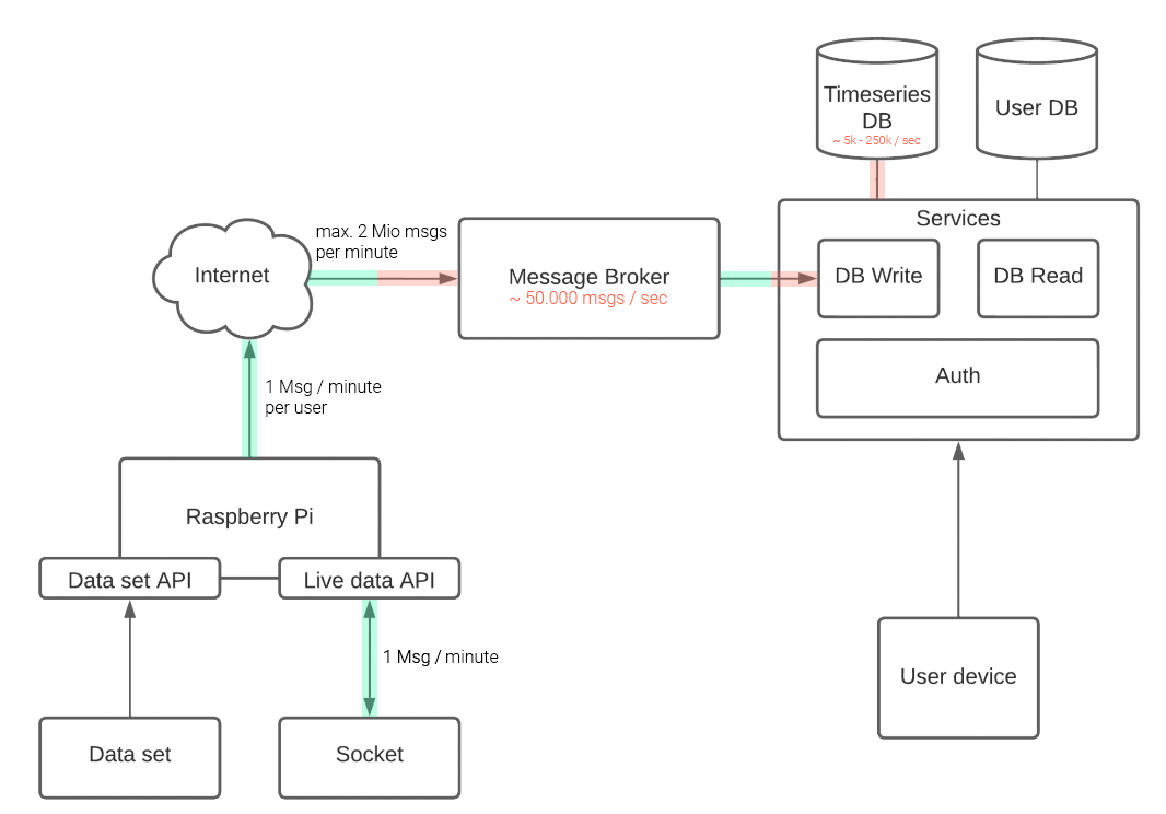
Fig. 4: Predicted bottlenecks in the systems components
To tackle the bottlenecks we listed some possible solutions for scaling and reducing the overproportional utilization of single components. Some of them included specific load balancing instances, database sharding and spreading load over time.
Monitoring
Before we conducted a load test we made sure that we were able to see the utilization of the critical components in our system. We therefore implemented the ‘TICK’ stack.
Telegraf → Data collecting agent
InfluxDB → Time series DB
Chronograf → Data visualization
Kapacitor → (Data processing) & alerting

Fig. 5: Monitoring inside Influx DB’s ‘Telegraf’

Fig. 6: Monitoring inside Influx DB’s ‘Telegraf’

Fig. 7: Monitoring inside Influx DB’s ‘Telegraf’
We created different dashboards to monitor the current utilization and throughput, as seen above. To connect our own services we implemented logging while using a shared data format which can be easily read by Telegraf. This allowed us to add most of our components to the monitoring system.
Load Test
Initially, we were using JSON as our data format. However, due to the relatively large size of JSON messages, we decided to switch to Protocol Buffers (protobuf) instead. This was due to the promising smaller transmitting size of protobuf messages.
In our protobuf message, we utilized a container object which contained multiple measurements. Each measurement contained the measurement name, device ID, energy measurement, and timestamp. This allowed us to effectively and efficiently transmit multiple measurements in a single message while keeping the overall size of the message to a minimum. By utilizing protobuf and optimizing our message format, we were able to improve the efficiency and effectiveness of our data transmission process.


Fig. 8 General data format used for the application
In order to determine the potential traffic requirements of our system, we conducted measurements to assess the size of our messages. We found that a container object containing eleven measurements was approximately 470 bytes, while a single measurement was around 37 bytes. We also measured the improvement in size comparing the container object in JSON and in protobuf. For JSON we measured that a container had the size of around 1075 bytes and thus our improvement in size was about 50%, which in network throughput can go a long way.
Using this information, we calculated the amount of traffic that would be required if we were to scale up to 2 million messages per minute, each containing a container object. Breaking it down to seconds would mean we had to scale up to 33 thousand messages per second. With this calculation, we were able to gain insight into the potential traffic demands that our system might face at scale. The expected amount of traffic required for our scale was expected to be around 14.95 MB/s, in regards to network traffic this would be around 119.6 Mbps. Knowing the network requirements and the shortcomings of slow home networks upload performance in Germany we were required to conduct load tests either with combined forces of several home networks or to test on the virtual machine itself or at least from within the same local network. We then tried the same machine approach.
Our general approach to load testing the system involved deploying it on our virtual machine and conducting performance tests. Initially, we tested the system as a whole but found that its performance was not meeting our expectations. To identify the root cause, we checked our monitoring and validated the performance of RabbitMQ both as a standalone component and as a part of our write service.


Fig. 9: Load testing the whole system and load testing the message broker
To conduct our load tests we used the RabbitMQ Performance Test Tool (perftest). Simulating the traffic from several Raspberry Pi instances from our system architecture.
| RabbitMQ Standalone | |||
| Data | 470 bytes | Our data | Our data |
| Ack | Auto | Auto | Manual |
| Producer | 2 | 2 | 2 |
| Receiver | 4 | 4 | 4 |
| Send rate Messages/s | ~51.000 | ~46.000 | ~21.000 |
| Receive rateMessages/s | ~50.000 | ~45.000 | ~20.000 |
The default PerfTest result for the RabbitMQ Standalone is higher than with our dataformat. This is probably due to the internal workings of the performance tool. As for the difference with RabbitMQ Standalone versus Standalone with manual ack there’s a large difference in over 50% performance loss. Going for throughput would mean that we would have to drop our data consistency.
| Full Application (RabbitMQ, WriteService & InfluxDB) | ||||
| Data | Our data | Our data | Our data | Our data |
| Ack | Manual | Auto | Manual | Auto |
| Producer | 2 | 2 | 2 | 2 |
| Receiver | 1 | 1 | 4 | 4 |
| Send rate Messages/s | ~10.000 | ~20.000 | ~13.000 | ~20.000 |
| Receive rateMessages/s | ~5.000 | ~19.000 | ~6.000 | ~20.000 |
For our application we see an even further decrease in messages per second. Using auto ack and four receiving threads we only achieved half the performance of the receiver from the testing tool. Also the amount of threads used for our Go application did not seem to make any difference for the throughput. For scaling we thus should rather deal with missing data and interpolation techniques.
Achieving only half the performance kept us wondering, which is why we took a look on our monitoring dashboards. At first glance either the WriteService or InfluxDB somehow became our bottleneck.

Fig. 10: InfluxDB writes during load test
The InfluxDB dashboard clearly shows a write peak of ~61.000 writes per seconds around the performance test.
Looking at the dashboard for our RabbitMQ we can see the performance around 20k messages per second as stated before. A slight difference is visible between ack and delivery rate of around 400 messages per second. Also the amount of acked messages did not match the messages sent through RabbitMQ. The amount of acked messages is equivalent to 11 * 20.000 ⇒ 220.000 rows per second, which our InfluxDB clearly didn’t reach.
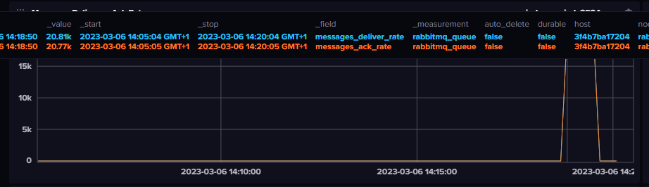
Fig. 11: Queue deliver and ack rate during load test.
We could see that we also validated the performance of our write service and InfluxDB, which led us to determine that the write service and InfluxDB were slowing RabbitMQ down. We then conducted additional tests to validate the performance of the write service in isolation.

Fig. 12: Load testing the Timeseries DB component
Using a customized Go client we conducted a write test outside our application. Writing 2 million data points first single threaded and then multithreaded to check if any performance gain is reached. We reached similar speeds leading us to the conclusion that our Go client might not be the issue. InfluxDB now being our main suspect of performance loss. Due to the custom testing tool we also discovered that using the convenience of the Point data object from the InfluxDB Go client library actually cost us time. Internally of the Go library the Point data object was just converted to the InfluxDB line protocol format. Removing the transformation from protobuf to point but instead writing line protocol ourselves we increased the performance of our writes.
Despite our efforts even when matching the throughput of InfluxDB to our RabbitMQ we could not have accommodated our use case of 2 Million users with 30 devices per minute. Achieving 46.000 messages per second for 11 metrics we would expect around 15.000 for 30 metrics per second. Scaling this to a per minute metric would mean that we can support up to 900.000 households which is roughly the half of our goal. So either way more improvements would be required for RabbitMQ and InfluxDB to reach our target.
Scaling
Our focus during system optimization was primarily on RabbitMQ, which resulted in neglecting the optimization of our writes to InfluxDB. As we were more accustomed to relational databases, we were unaware of the performance relevant configurations of InfluxDB. Our load tests revealed that the main issue was with our writes to the database, but we cannot be certain if we have optimized our single InfluxDB instance to its full potential.
Given our VM constraints, it would have been better to place InfluxDB on a separate VM with an SSD and more RAM for better write performance. Additionally, we should have revisited our write design of the Go client, which we then could have verified with InfluxDBs own performance test tool called Inch. Moreover, we could have considered using multiple InfluxDB instances/sharding to further increase our write performance.
For RabbitMQ we would have required scaling as well, maxing our throughput for a single instance an improvement only could have been made with more instances and load balancing.
Unfortunately, most of these options were out of scope for our student project, but they can be explored with more time and computational resources.
Lessons Learned
Monitoring & Error search
Right from the beginning we were aware that running our observability solution on the same system we want to monitor is a bad idea. If there were a complete system outage there would be no way for us to see what happened as the monitoring would crash along with the system.
We did it anyway because we were limited to our single VM on which we needed to deploy our entire application. We expected that we were not going to be able to monitor our system during network outages, deployments, etc. However, what we hadn’t fully considered is that this would also cause problems for us when trying to evaluate the performance of our services during the stress tests.
While performing a stress test, our Chronograf dashboards would first become slow and unresponsive because the system was under so much load. What we were able to see though was that the RabbitMQ and our write service would slowly eat up the entire system RAM, at which point the monitoring would only report back errors and Chronograf became completely unreachable. We did not anticipate that the other components would start stealing resources from our observability stack. Then again, part of that very stack, our InfluxDB, was being stress tested, which explains why the monitoring became slow to update.
All this supports our plan to run the monitoring on and as a separate system in a market-ready version of the application.
Monitoring was also somewhat handy in finding bugs in our application: At one point our write service reported CPU usage of over 180 %. This was a clear indicator that there was a bug in our implementation. Thankfully though, it was just putting high demand on the CPU at that moment and hadn’t crashed our system yet. We rolled the service back to an older version where the bug hadn’t been observed, which gave us the time to find and fix the bug and quickly deploy the updated version without causing substantial disruption to the application.
This, we think, is an excellent example of how monitoring paired with alerting can prevent outages or at least minimizes downtime.
Development Process
Despite reaching a solution that works, there are quite a few things where we struggled along the way. Some of the lessons almost feel like they’re part of a book entitled “Wouldn’t it be cool… and other bad design approaches”. Making these mistakes can be embarrassing to admit, but struggles always bring an opportunity to learn with them.
In retrospect, we lost ourselves in creating too much unnecessary functionality too early in the project. An example would be attempting to create a sharding resolver that lookups user tokens to distribute writes across different influx instances and buckets. Deep down we knew that it would probably be out of scope but we still fell victim to our curiosity. The proper way would have been to implement a minimal working prototype first, conduct a performance analysis, identify the bottleneck, and only then spend resources to resolve it.
While we recognize that anticipation of future problem sources is a valuable trait in developing software, not being able to resist these impulses massively harms overall productivity. In our case this meant we were constantly switching between problems, creating more and more zones of construction in the process. This made it harder to orient in the code and difficult to decide what to work on next.
What is so frustrating is that we are aware of this tendency and know the solution is to practice an iterative and incremental approach to development, yet we tend to repeat these rookie mistakes. Unfortunately, we realized too late that hexagonal architecture has a natural workflow to it that helps with the problem of getting lost. First, you start by getting a clear understanding of the problem domain. We recommend using draw.io to sketch out the components of the application and how they interact. Next, you define the application’s ports. Ports should be defined upfront, as they represent the key abstractions of the application and ensure that the application is designed to be technology-agnostic. The definition of port interfaces often happens in unison with the definition of domain objects, because domain objects inform the design of the interface and are often used as input and output parameters. Once ports are defined, develop the core business logic of the application. After that, it is a good practice to test the core business logic to validate it meets the functional requirements of the application. Testing the business logic before implementing the adapters also helps to ensure that any issues or bugs in the core functionality of the application are detected and resolved early in the development process.
Once the business logic is implemented and tested, proceed to implement the adapters that connect the application to the external environment. Test the adapters to ensure they conform to the ports and correctly transform data between the external environment and the business logic.
After adapters are implemented and tested, you can test the system as a whole, to ensure that all components work together as expected. This testing should include functional and integration testing. Last, refactor and continue to improve the design. In comparison, our unstructured and unfocused approach to implementation cost us valuable time.
Without following the workflow described above, you tend to push testing towards the end of the project. The combination of having acquired debt (need to re-factor code to make it easier to test) and a self-inflicted lack of time meant, we were not able to take advantage of hexagonal architecture offers in the domain of testing.
| func WriteEvent(msg interface{}, target interface{}) error { // let the type checks begin … } func WriteWattage(m *domain.WattageMeasurement, token string) error { // no such problems } |
Fig. 13: Different approaches with very generic interfaces (top) and specific types (bottom)
Another problem we encountered was finding the right degree of abstraction. A generic solution is typically designed to be flexible and adaptable so that it can be used in a wide range of use cases without requiring significant modification. These adjectives sound highly desirable to the ears of a developer and, as a result, we wanted to build our code in a way that would allow completely changing out the message format, inject adapters via configuration instead of touching the source code, etc. It’s fair to say that my initial implementation was way too generic. More and more it felt like we were not building a solution to our specific use case, but almost a framework that could be used for similar problems. Eventually, we realized that generic doesn’t mean good. Adding lots of adaptability naturally adds more abstraction and indirection to the code. The most glaring indicators that something was going wrong were that our interfaces were inexpressive/vague, exhibited weak type safety, and forced us to write unnecessary code complexity to deal with that. When you build a highly adaptable system that can adapt to a whole bunch of cases that never happen, then all of that just ends up being a big waste of time. In hindsight, it is difficult to analyze what caused this obsession with developing something generic. Once we re-wrote everything to be as specific to our problem domain as possible, the code became expressive and readable, and the need for using empty interfaces as function parameters vanished.
Identifying and improving bottlenecks
As software developers, we’ve all experienced the frustration of trying to identify and resolve bottlenecks in a system. We know that while it’s easy to detect the general location of a bottleneck, it can be hard to determine the actual issue. It’s also challenging to predict how software will perform with different hardware specifications or how all the components will interact with each other on a virtual machine. As we had no knowledge of the actual performance on our virtual machine we started to put everything on the machine and first tested the system as a whole. While the approach can work it is harder to determine the actual issue when a bottleneck seems to be prevalent. Also, using the numbers provided by the software vendors for the software solutions can help to get a rough estimate of the performance; it’s still different with each use case and current set up and can’t replace making your own measurements when going for performance.
One valuable lesson we’ve learned is to take a more methodical approach to identifying bottlenecks. Checking first if there is a load testing tool to produce load for a single component and then verifying the results with a custom implementation. For our approach as soon as we noticed a bottleneck we started to check each component individually on the target machine before adding additional components. This helped us isolate the source of the issue. Without our monitoring in place we would never have detected the bottleneck and we’ve thus realized that monitoring is crucial in detecting performance issues. By tracking performance metrics, we could identify areas of concern and take action to optimize processes such as unnecessary convenience data transformations and, depending on the use case, unrequired data consistency, which can significantly impact system performance.
In summary, while the process of identifying and resolving bottlenecks can be challenging, we’ve learned that taking a structured approach and paying close attention to performance metrics can help us identify and address issues efficiently.
Leave a Reply
You must be logged in to post a comment.