What this blog entry is about
The entry bases on the paper “The Essential Guide to Queueing Theory” written by Baron Schwartz at the company VividCortex which develops database monitoring tools.
The paper provides a somewhat opinion-oriented overview on Queueing Theory in a relatively well understandable design. It tries to make many relations to every day situations where queueing is applied and then provides a couple of annotation methods and formulas as a first approach to actual calculations.
This blog entry forms a summary of that paper but focuses on queueing in the context of ultra large scale web services and adds examples and information from my own knowledge and trivial research.
The goal of this blog entry is to provide fellow computer science and media programmers who consider working in the field of web servers an overview about queueing that might be helpful at some point to understand and maybe even make infrastructure- and design-decisions for large scale systems.
Note that some annotations do not match exactly to the paper from Schwartz because there seems to be no consensus between it and other sources either. Instead the best fitting variants have been chosen to fit this summary.
Queueing and intuitition
The paper sums up the issue as “Queueing is based on probability. […] Nothing leads you astray faster than trusting your intuition about probability. If your intuition worked, casinos would all go out of business, and your insurance rates would seem reasonable.”
Due to the skills required for survival in prehistoric times as well as due to most impressions we make nowadays in everyday life, the human mind is best suited for linear thinking. For example the Neanderthal knew that if he gathers twice as many edible fruits, he will eat off them twice as long (just imagine yourself today with snacks in the supermarket : ) ).
An exception to this is movement prediction where we know intuitively that a thrown object will fly a parabolic path. This part already comes to a limit though when we think for example of the famous “curved free kick” (Keyword: Magnus effect).
However when we try to think theoretically about things in our mind alone, we tend to resort solely to linear proportions between two values.
As we will see and calculate later, in queueing theory, relations are not just parabolic but unpredictably non-linear. A value can grow steadily for a long while until reaching a certain point and then leap rapidly towards infinity.
Let’s look at an example: You have a small web-server providing a website that allows the user to search and display images from a database.
Depending on how broad the search is, preparing and sending the search-results to the user takes a random amount between one and 3 seconds – on average that means 2 seconds. Also on average you expect 25 customers per minute.
Now the question is, how long will the user have to wait on average?
Intuitively (at least if you would not be a software dev ; ) ) you might say: Barely over two seconds. After all, handling 25 requests of 2s average each, requires just 50 seconds and thus only 5/6 (83.3%) of the systems time.
Unfortunately the reality would be a website with 5 seconds of wait time on average and far higher outliers.
The reasons are that with random request processing duration as well as random arrival time, request will naturally overlap and waiting time is automatically wasted. Whenever the server has no request to handle, those seconds are entirely lost. When multiple requests occur simultaneously later, it is not possible to “use up” that spare idle time from earlier. Instead time continues to flow and the requests have to be enqueued and wait.
The following graph shows the relation between “Residence Time” which is the whole time between arriving with a request and leaving with it (aka the site loading time) and “Utilization” of the server.
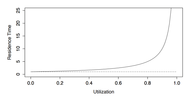
We see a non-linear graph that is sometimes called “hockey stick graph” due to its markant shape. It shows well how the tipping point is somewhere around 80%. Past this amount of utilization, average wait time skyrockets.
The Residence Time and Utilization are only two of several values that we need to define to be able to talk on a common ground about queueing theory.
The common ground
To form a base of words and abbreviation see the following table.
| Metric | Unit | Symbol | Description |
| Arrival Rate | Requests per time | A | The frequency of new requests to the system. |
| Queue Length | Waiting requests | Q | How many requests are waiting in a queue on average. |
| Requests (in concurrency) | Requests | R | Total requests currently waiting or being serviced. |
| Wait time | Time | W | Time requests spend waiting in a queue |
| Service time | Time | St | Time a request needs to be serviced on average. For example how long it takes to assemble the website data. |
| Residence time (latency) | Time | Rt | Total time from placing the request and returning the output. If ignoring data transfer delays, this naturally is W + St. |
| Utilization | Fraction | U | Percentage of utilization of the servers. Refers to the quote of busy-time from the total time. It’s reciprocal is the idle-time. |
Basic formulas
Many of the parameters listed above are related to each other through a handful of basic formulas that are mostly trivial once you understand them.
The first and most common one is referred to “Little’s Law” as it has been formulated and proved in 1961 by John D.C. Little:
R = A * Rt
Where R is the number of total requests in the system (in queue and currently serviced), A the arrival rate and Rt the total time of a request from arrival to having been serviced.
The relation is fairly straight forward as it simply says, the longer requests take in the system and the more often they occur, the more requests will accumulate in the system.
This relationship can be resolved for the queue length as well:
Q = A * W -> Queue length = arrival rate * wait-time in queue
Another important formula is the Utilization Law:
U = A * St -> Utilization = arrival rate * service time of a request
Logical; the more services arrive and the longer time they need to be serviced, the higher utilization will be on average. To calculate this for multiple servers, just divide the utilization by servers. Of course this is for the theoretical approach only as real web servers will inevitably have an overhead through load balancing.
Last we have another important formula that says that the residence time Rt which is the latency of a request, is equal to the service time divided through the idling-percentage of the servers (1 – utilization).
Rt = St / (1-U)
Those formulas however do not allow you to predict much of how a real system will behave yet because they require you to know at least one crucial thing like average queue length, wait time in queue or the utilization.
To compute any of those, a more advanced set of formulas are needed. However before we can calculate something for a system, we first need to decide how to describe such a system.
Kendall’s annotation
A way to fulfill exactly that and describe approximately how a service system has been designed, is the “Kendall’s annotation”. It allows to differ between systems by major parameters.
Up to six parameters, each anotated by a letter, are separated by dashes:
A/T/S/P/R/D
Unfortunately the exact letters for every parameter differ a lot between sources. Therefore this blog entry describes a variant that appeared senseful to the author. Most sources use exactly the same order of parameters though.
Of all parameters, the first three are most significant as the others can be their default values for many systems.
A
The first parameter describes with what behavior the service-requests arrive. Most commonly that is one of the following letters:
- M or G: Memoryless or General; means the requests occur randomly (there’s no memory of the last request). This results in an exponential distribution.
- Mx: Random occurence of x requests at once.
- D: Degenerate distribution; A deterministic or fixed time between requests
- Ek: Erlang Distribution; Erlang Distribution with k as the shape
T
T describes the service time distribution. The same letters as for (A) are common.
S
S describes the number of services that serve requests in parallel.
P
P denotes the number of places in the system including services and queues. When this limit is reached, new requests are denied.
If omitted, this parameter is ‘infinite’ (INF).
R
R is the number of possible requesters. This is only relevant if the number of requesters is relatively low because if a significant fraction is already in queues, new requests naturally become more scarce.
If omitted, this parameter is ‘infinite’ (INF).
D
D describes the de-queueing behavior. The following abbreviations are common:
- FIFO: First in first out
- LIFO: Last in first out
- SIRO: Service in random order
- PNPN: Service order based on a priority value for every request
If omitted, this parameter is ‘FIFO’ by default.
Example
Following the Kendall’s annotation, a possible variant of a web service system is:
M/M/(s)/(b)/INF/FIFO
Where (s) is the number of requests that can be processed in parallel and (b) is the number of places for requests in memory in total.
A service system described like that means it expects requests at random intervals* and each requiring random time to process. It expects an infinite number of potential requesters because even for the largest system it is not feasible to be able to handle a significant fraction of all people with internet access at the same time**. It utilizes FIFO queues.
* Of course a system can make predictions like higher demand on certain times on the day, but that is not immediate enough because it is not a correlation between two requests. However for some types of sites (like social media for example) it can be assumed that after a user has accessed the first time, subsequent requests will occur as he keeps using the site. This type of behavior cannot be modelled with Kendall’s annotation.
** However for services available only to special, registered users the number may be limited.
Predicting the Behavior of single-server designs
A major point about those relatively theoretical approaches at queueing systems are the possibility to make certain predictions about their behavior in practice. The two numbers of interest are queue length and wait time.
In the context of the service of a large scale system, the queue length is relevant to determine the required memory for the system (or every particular machine).
The wait time on the other hand is significant for the user’s satisfaction with the whole service.
Indirectly the results of those predictions determine the required performance of the system to avoid an utilization that results in high waiting times (both tending towards infinity) as seen in the “hockey stick graph” earlier and usually in high queue lengths as well.
First it makes sense to look at the formula generating said graph for a queue that has the Kendall annotation M/M/1. That means it has random request- and service time, infinite requesters and queue-memmory and unitlizes a FIFO principle. That all runs on a single server.
The formula is:
R = S / (1 – U)
Where R is the total wait time (“residence time”), S the service time and U the utilization of the server.
Following this, the residence time is proportional to 1/(1-U). That’s often referred to as the stretch factor because it describes how much the real total wait time is stretched compared to the time needed to process a request after it left the queue.
Try out the formula here with this interactive online tool (U has been used as x and R as y).
You will notice that the lower S is, the more the critical percentage of utilization can be put off. As a rule of thumb the following can be deduced: Halving the idle capacity, doubles the whole, average response time!
Using the graph formula together with “Little’s Law” mentioned earlier, it is possible to compute further values related to the queue:
R = U / (1-U)
Where R is the average number of customers currently in the system (in queue and currently serviced).
Q = U² / (1 – U)
Where Q is the average queue length.
Eventually the time W requests wait in a queue before being serviced can be computed on average as:
W = U*St / (1-U)
Where St the service time and U the utilization of the server.
Predicting the behavior of multi-server designs
The “correct method”: The Erlang formulas
Agner Erlang who pioneered in the field of telecommunications formulated a series of equations in his field. For example one to predict how many telephone lines would be needed to carry an expected volume of calls.
A modern form of the formula involves the unit nowadays known as “Erlang” that describes the service demand. Indirectly the amount of Erlang is equal to the amount of concurrency in the optimal case and therefore the number of servers required to handle all requests.
A practical example are the backbone-telephone lines. Naturally one telephone line can “service” 60 minutes of talk in one hour. That results in exactly 1 Erlang.
Now if the real requests sum up to 600 1-minute calls in one hour, that results in 600 minutes of talk and therefore 10 Erlangs.
In practice of course a backbone with 10 lines and said demand would mean that calls would often need to wait for a free line.
This is where Erlang’s formula ‘C’ comes into play:
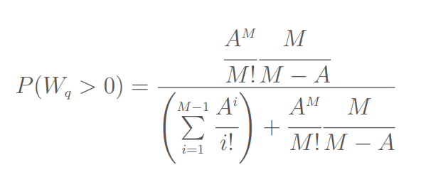
This massive, internally iterative formula calculates the probability that a new request has no free line and therefore has to wait in a queue.
A is the request load (the current demand) in Erlangs and M is the number of total servers (or telephone lines in this example).
Wolfram Alpha allows to see this formula in action.
As expected, for the edge-case of 10 Erlang of demand and 10 available servers, the probability that the new request has to wait is practically 100% because the probability that all calls coincidentally line up accurately one after another is negligible low.
With 11 servers or telephone lines that result in a system that allows more overlapping, the result of the Erlang C formula is already about 68%.
Applying “Little’s Law” it is again possible to derive different formulas to compute desired values, however Erlang’s formulas are not easy to apply and very unintuitive. For this reason, an approximation has been found.
The aproximated method
For the case that there is one waiting queue but Xs servers, a modification of the earlier basic formula can be used:
Rt = St / (1-U^Xs)
Where S is still the service time and U the utilization.
By applying the number of servers as an exponent to the utilization, the formula is equal to the old formula in the case of 1 server. Furthermore for other cases it results only in an underestimation of total request time of up to 10%. More information can be found in Cpt 2 of “Analyzing Computer System Performance With Perl::PDQ (Springer, 2005)” by Neil Gunther.
One common queue or one queue per server?
Using the formulas, the answer to this question is always that a single queue is more efficient. The logical reason becomes clear if we keep in mind that processing requests also takes random amount of time. This can result in a situation where one server is occupied with a large request while the other server has handled its whole queue already and now has to idle.
This is why server infrastructure tends to use “load balancers” that maintain a queue of user requests and spreads them to servers.
However because transmitting requests from the balancer to a server is taking time too, the servers usually hold queues themselves to ensure to be able to work constantly.
Nevertheless, sophisticated algorithms are required for load balancers to ensure a stable system especially under unusually high load or when servers drop out. This topic is handled in other blog entries.
You can experiment with the Erlang C formula modified to compute the residence time depending on the number of servers here.
This shows how a higher number of servers also allows for better utilization of the whole system before the wait time rises too much.
Problems and Limitations
Certain precautions have to be taken before the computations above can be used in a reliable way.
Exact measurements
The two key values of the system, service time S and current utilization U need to be known accurately. This can be tricky in server environments where random network- and infrastructure-delays are added under certain circumstances or where servicing can require waiting on other, secondary services (common nowadays when building serverless websites).
A quality measure of modern server management systems are the ability to determine this and especially the utilization of the system.
Ensuring exponential distribution
While this is typical, it has to be ensured that service times do spread sufficiently close to an exponential distribution.
Cross-dependency
Modern websites are often built “serverless” and require assembling data from different sources. It is possible to assume an abstraction and only view the desired layer of services (like only the outer that delivers to the users, or for example the system inside that delivers only the images to the other process that assemble the website). However things become less predictable when a sub-service utilizes a resource that is currently needed by a different request.
Conclusions
Due to those reasons, the authors of the major paper this blog entry is based on, suggest that the queueing theory described above is most suited for everyday and physical problems. There they can be applied for relatively simple decisions. Additionally they can be used to find possible problem-causes when an actual system does not behave as assumed. In the end they mainly help to adjust peoples personal intuition that often is wrong due to the non-linearity of relations in queueing problems.
Personally I find that knowing about queueing theory and having experimented with the formulas can indeed open ones eyes to what is actually predictable and what is not. Furthermore together with modern observation tools for server systems, I would definitely suggest trying to apply the concepts and formulas to verify whether a certain system is working in an optimal way or not. Last but not least they can form a starting point when beginning to design a server infrastructure.
Leave a Reply
You must be logged in to post a comment.