Gigantische Datenmengen auf der DNA

14. February 202314. February 2023 ~ Rebecca Westhäußer

Ein Artikel von Michelle Albrandt, Leah Fischer und Rebecca Westhäußer.

Durch die Digitalisierung werden immer mehr Daten erzeugt. Dabei erreicht die Datenbasis durch Vernetzung von Mensch zu Mensch, sowie auch von Mensch zu Maschine, eine neue Dimension (Morgen et al., 2023, 6). Prognosen für das Jahr 2025 zeigen, dass in Zukunft ein erhebliches Datenwachstum zu erwarten ist, wobei insgesamt 181 Zettabyte an Daten erzeugt oder repliziert werden sollen (Tenzer, 2022). Aber nicht nur in Zukunft muss mit Herausforderungen gerechnet werden. Dies zeigt ein Vorfall des Erdbeobachtungsprogramms “Sentinel”.Das Earth Observation Center (EOC) verwaltet und archiviert die Daten der Satelliten und hat im Januar 2019 die maximale Speicherkapazität überschritten, wobei erstmals der Wert von 10 Petabyte überschritten wurde, was 10 Millionen Gigabyte entspricht(Earth Observation Center – 10 000 000 Gigabyte Sentinel Am EOC, 2019).

Mit der Zunahme der hohen Datenmengen steigt demnach auch die Nachfrage nach Datenspeicherlösungen mit großer Kapazität. Herkömmliche Speichermedien müssen aufgrund ihrer kurzen Lebensdauer regelmäßig ausgetauscht werden (Welzel et al., 2023, 1). Beispielsweise beträgt die Lebensdauer für Festplatten 10 Jahre und für Magnetbänder 30 Jahre. Zusätzlich haben solche Medien eine begrenzte maximale Informationsdichte von etwa 10³ GB pro mm³, wie beispielsweise bei Festplattenlaufwerken (Konitzer, 2021, 4). Durch Häufigkeit der Schreib- oder Lesezugriffe kann sich die Lebenszeit sogar verkürzen. Lesezugriffe sind zur Überprüfung der Datenintegrität jedoch notwendig (Potthoff et al., 2014, 14).

Ein langfristiges Speichermedium muss aber nicht neu entwickelt werden. Das beste Beispiel für Datenspeicherung, die nahezu ewig anhält, ist eines der allerersten Speichermedien überhaupt, die DNA. DNA kann sehr lange bestehen. So war es möglich, 2015 das Genom eines Wollmammut zu sequenzieren. Dies gelang den Forschern, obwohl der gefundene Knochen 4000 Jahre alt war (Konitzer, 2021, 4). Informationen nicht nur zu extrahieren, sondern auch in der DNA zu speichern, hatten Forscher bereits in den 60er Jahren vor. 50 Jahre später ist es in zwei unterschiedlichen Gruppen gelungen, Daten in Größe von einem Megabyte in der DNA zu speichern. Nach erfolgreichen Errungenschaften, wie ein robustes DNA-Datenspeicherung System durch Fehlerkorrektur und dem Nachweis einer hohen Informationsdichte (2 Bit pro Nukleotid), wurde im Jahr 2018 eine Speicherkapazität von ca. 200 Megabyte erreicht, wodurch das Potenzial dieser Vision immer realistischer wurde (Shamorony & Heckel, 2022, 4).

Datenspeicherung auf der DNA

Um zu verstehen, wie Informationen auf der DNA gespeichert, konserviert und wieder ausgelesen werden können, muss zunächst die Struktur der DNA angesehen werden. Die Desoxyribonukleinsäure, kurz DNA, besteht aus Basen, Desoxyribose (Zucker) und einer Phosphatgruppe und ist Träger der genetischen Information des Menschen. Es gibt vier verschiedene Basen: Adenine, Guanine, Cytosine und Thymine. Eine Base bildet zusammen mit einem Phosphat und einer Desoxyribose ein Nukleotid. Mehrere Nukleotide aneinandergereiht bilden einen DNA-Strang. Die bekannte Doppelsträngige Helixform der DNA wird durch die Verbindung der komplementären Basen Adenin und Thymin sowie Guanin und Cytosin gebildet. Die Abfolge der Basen stellt die codierte Information dar. Dies ermöglicht die Speicherung von Daten auf der DNA, indem diese in den genetischen Code übersetzt werden (De Silva & Ganegoda, 2016, 2-3). Infolgedessen muss DNA geschrieben und wieder ausgelesen werden. Dieser Vorgang wird als Synthese und Sequenzierung bezeichnet (Hughes & Ellington, 2017, 1).

Kodierung

Es gibt bereits viele verschiedene Methoden zur Kodierung der Daten. Im Allgemeinen funktionieren sie jedoch alle nach dem gleichen Schema. Zunächst wird der Binärcode der Dateien in quaternäre Zahlen aufgeteilt. Das bedeutet, dass jeweils vier aufeinanderfolgende Nullen und Einsen des Binärcodes zusammengefasst werden. Jede Base entspricht einer quaternären Zahl, wodurch der binäre Code in den genetischen Code übersetzt werden kann. Dieser Schritt wird als Source Coding bezeichnet. Zur Kodierung von Textdateien können zum Beispiel folgende Methoden verwendet werden: arithmetische Kodierung, Wörterbuch-Kodierung oder Huffman-Kodierung. Von den genannten Beispielen ist die Huffman-Kodierung sehr populär in der Anwendung. Hier werden häufig vorkommende Symbole mit einer kurzen Codierung und selten vorkommende Symbole mit einer längeren Codierung versehen. Dadurch wird die durchschnittliche Länge des Codes für den zu speichernden Text reduziert. Auf diese Weise wird gleichzeitig die zu speichernde Datenmenge komprimiert, was einen weiteren Vorteil darstellt. Darüber hinaus sind alle Sonderzeichen in der Kodierung enthalten (Dong et al., 2020, 1096-1098).

Informationsfluss in der DNA-basierten Informationsspeicherung (In Anlehnung an (Dong et al., 2020, 1096))

Die Kanalcodierung wird verwendet, um die Informationen vor Verzerrungen während der Übertragung zu schützen. Solche Verzerrungen können beispielsweise bei der Synthese oder der Sequenzierung auftreten. Um die Informationen vollständig wiederherstellen zu können, wird Redundanz erzeugt. Die Redundanz kann entweder physisch oder logisch sein. Physikalische Redundanz entsteht durch die Anfertigung von Kopien desselben DNA-Strangs, so dass es mehrere Kopien mit der gleichen Information gibt. Bei der logischen Redundanz hingegen werden sogenannte Prüfzeichen hinzugefügt, um Fehler erkennen und korrigieren zu können. Mit der Basenfolge, in der die Informationen enthalten sind, kann nun eine synthetische DNA erstellt werden, die demzufolge ebenfalls die zuvor kodierte Information enthält (Dong et al., 2020, 1096-1098).

Lagerung/Speicherung

Da DNA zum Beispiel durch UV-Strahlung, Wasser oder Enzyme zersetzt wird, muss sie geschützt werden, damit die auf ihr gespeicherten Daten nicht verloren gehen. Während die Halbwertszeit der DNA in Fossilien und unter perfekten Bedingungen mehrere 100 oder gar 1000 Jahre beträgt, verschlechtert sich dieser Wert drastisch, wenn die DNA Feuchtigkeit ausgesetzt wird (DNA DATA STORAGE ALLIANCE, 2021, 27). Synthetisierte DNA kann in vivo oder in vitro gelagert werden (Dong et al., 2020, 1096). Der Begriff “in vivo” kommt aus dem Lateinischen und bedeutet “an einem lebenden Objekt”, während “in vitro” “im Gefäß” bedeutet. Daraus folgt, dass bei der in vivo DNA-Speicherung die DNA in einem lebenden Organismus enthalten ist. Bei der in vitro DNA-Speicherung wird die DNA außerhalb eines Organismus gespeichert (Elder, 1999 & von Reininghaus, 1999).

Als eine der besten Varianten für die Speicherung von DNA gelten Sporen (Cox, 2001, 247). Sporen sind einzellige Fortpflanzungsorgane und -einheiten in Pflanzen und Pilzen (Sporen – Lexikon der Biologie, n.d.). Sie werden als eine sehr gute Möglichkeit angesehen, da sie auch unter sehr lebensfeindlichen Bedingungen überleben können und daher auch nach mehreren Millionen Jahren noch abrufbar wären. Außerdem vermehren sich die Sporen selbst weiter und erzeugen so automatisch Kopien der gespeicherten Daten. Für zusätzlichen Schutz können die Sporen in Bernstein eingeschlossen werden (Cox, 2001, 247).

Zu den möglichen in vitro Methoden für die längerfristige Lagerung von DNA gehören der molekulare und der makroskopische Schutz. Bei der so genannten chemischen Verkapselung wird der molekulare Ansatz verwendet. Dabei werden die einzelnen DNA-Moleküle in ein Matrixmaterial eingebettet, das die Diffusion von Wasser und Sauerstoff zu den einzelnen DNA-Molekülen verhindern soll. In den meisten Fällen bestehen die Matrizen aus anorganischen Materialien wie Glas. Beim makroskopischen Ansatz wird die DNA getrocknet und in Gegenwart eines reaktionsträgen Gases, beispielsweise in einer Metallkapsel, gelagert. Dieses Verfahren wird auch als physikalische Verkapselung bezeichnet. Solange die Unversehrtheit des Behälters gewährleistet werden kann, lassen sich chemische Reaktionen der DNA-Moleküle vermeiden (DNA DATA STORAGE ALLIANCE, 2021, 28).

Vor- und Nachteile

Die Datenspeicherung in der DNA hat viele Vorteile, die die DNA zur Zukunft der Datenspeicherung machen. Der größte Vorteil ist die parallele Berechnung. Mit der DNA können viele Operationen gleichzeitig ausgeführt werden, was bedeutet, dass die Leistungsrate sehr hoch ist. Hinzu kommt die effiziente Nutzung von Speicher und dem verfügbaren Platz. Beispielsweise passen rund 10 Billionen DNA-Moleküle auf einen Kubikzentimeter, was theoretisch einem Computer mit 10 Terabyte Speicherplatz entspricht (El-Seoud & Ghoniemy, 2017). Ein weiterer positiver Aspekt sind die geringen Energiekosten für die korrekte Lagerung im Vergleich zu herkömmlichen Speichermedien. Sie kann Jahrtausende lang überleben und ist zudem wesentlich umweltfreundlicher, da sie biologisch abbaubar ist und für die Erzeugung keine Schwermetalle oder seltene Elemente verwendet werden (Zhirnov et al., 2016).

Neben den genannten Vorteilen gibt es auch Nachteile, die die Nutzung der DNA mit sich bringt. Zum einen ist die Arbeit mit massiven Datensätzen ein Nachteil, da hierbei die Fehlerwahrscheinlichkeit exponentiell ansteigt. Zudem stellt die Analyse der Ergebnisse Schwierigkeiten dar, da es sich um Milliarden von Molekülen handelt, die miteinander interagieren (Akram et al., 2018). Der Durchsatz beim Lesen und Schreiben von Daten ist ein weiterer Nachteil sowie die Kosten für die Speicherung, welche derzeit zwischen 800$ und 5000$ liegen (Meiser et al., 2022). Ein weiterer wichtiger Aspekt sind die anfallenden Kosten für die Labore und die biologischen Experimente, die durchgeführt werden müssen, um die Speicherung der DNA überhaupt zu ermöglichen. Der größte Vorteil ist zugleich auch ein Nachteil, da die parallelen Berechnungen extrem viel Zeit in Anspruch nehmen (El-Seoud & Ghoniemy, 2017).

Anwendungen

Es gibt zahlreiche Möglichkeiten, wie die DNA in Zukunft für Daten eingesetzt werden kann. Die Forschungen hierfür gehen in verschiedenste Richtungen, aber der relevanteste Aspekt ist die Speicherung von Daten. Erste Studien haben Daten mit einer Größe von 200 Megabyte auf der DNA gespeichert. Weitere Forschungen haben beispielsweise 2000 Bilder als Kunstwerk oder ein Musikalbum auf der DNA kodiert. Anfängliche Berechnungen der Forschungen zeigen, dass alle Informationen, die in einem Jahr global erzeugt werden, auf ca. 4g von DNA gespeichert werden könnten, was den Vorteil der optimalen Nutzung von Speicher und Platz der DNA verdeutlicht (Boyle & Bergamin, 2020 & 2018).

Eine Einsatzmöglichkeit von DNA als Informationsträger ist das Barcoding bzw. das sogenannte Product Tagging. Bisher sind Barcodes auf Produkten oder auch QR-Codes bekannt, allerdings können diese Codes beispielsweise nicht für Tabletten oder Textilien verwendet werden. Hierfür bietet die DNA die Lösung der molekularen Barcodes. Das ist eine feste Menge an DNA, die den Bausteinen von Substanzen hinzugefügt wird. Diese müssen über den ganzen Lebenszyklus des Produktes intakt bleiben und ungiftig sein. Anhand der molekularen Barcodes kann Information zu einem Objekt hinzugefügt werden, ohne dass es für das menschliche Auge sichtbar ist (Meiser et al., 2022).

Die Erweiterung des Barcoding und der Datenspeicherung ist die DNA of Things (DoT), was sich von “Internet of Things” ableitet. DoT ist eine Mischung der beiden Ansätze und kann beispielsweise für das Labeling von medizinischen Produkten genutzt werden oder auch für Materialien, die eine Produktkontrolle benötigen. Für die Kontrolle wird die Tatsache genutzt, dass die Information nicht sichtbar ist (Koch et al., 2020).

Weitere Einsatzmöglichkeiten der DNA sind beispielsweise ein Random Number Generator oder die Kryptografie, wobei versucht wird, eine Nachricht in der DNA zu verschlüsseln. Hier wird momentan an einem Ansatz geforscht, wo menschliche DNA mit der Nachrichten-DNA gemischt wird, um die Nachricht zu verschleiern. Jedoch hat auch dieser Ansatz sehr lange Lesezeiten, was momentan noch ein generelles Problem bei der Nutzung von DNA ist (Meiser et al., 2022).

Aktuelle Entwicklungen und Ausblick

Wissenschaftler, wie auch Unternehmen, sind sehr daran interessiert, diese Technologie zu perfektionieren und an den Markt zu bringen. Seit 2020 gibt es die DNA Data Storage Alliance (DDSA), welche sich dieser Disziplin stellt. Gründer sind Unternehmen wie Illumina, Microsoft, Twist Bioscience und Western Digital. Ziel des Bündnisses ist es, auf Basis von DNA als Speichermedium ein interoperables Speichersystem zu schaffen und dieses auch zu fördern. Dazu gehören Spezifikationen und Standards in Bezug auf Kodierung, physische Schnittstellen, Aufbewahrung und Dateisysteme, die im Rahmen der Forschung entstehen sollen (DNA DATA STORAGE ALLIANCE, 2021, 5).

Im Oktober 2022 veröffentlichte die DDSA konkrete Anwendungsfälle für Fahrerassistenzsysteme (ADAS). Potential sieht die Allianz daher, weil Fahrerassistenzsysteme durch Sensorik Unmengen an Daten produzieren. Hohe Raten sorgen dafür, dass autonome Fahrzeuge bei Spitzenauslastung etwa 15.000 Gigabyte in einem Zeitraum von acht Stunden erzeugen. Bei steigenden Autoverkäufen wird vermutet, dass im Jahr 2025 mindestens 400 Millionen vernetzte Personenkraftwagen unterwegs sein werden. Daraus entsteht ein monatlicher Datenverkehr von zehn Exabyte. In Zukunft wird die Geschwindigkeit der Datenerzeugung ebenso durch steigende Automatisierung und zusätzliche Sensorik beschleunigt. Gründe, die laut DDSA, für die Nutzung von DNA-Speichersystemen sprechen, ist der Bedarf an hochparallel Berechnungen zum Beispiel für eine Suche oder Musterabgleich, trotz langsamer Leselatenz. Andere Archivierungsanforderungen für ADAS wie eine hohe Kapazität, belastbare und unveränderbare Speicherung mit niedrigem Total Cost of Ownership sprechen ebenfalls dafür (DNA DATA STORAGE ALLIANCE, 2022, 6-13).

Es ist sicher, dass die Speicherung von Daten auf der DNA ein großes Potenzial aufweist. Jedoch müssen für den alltäglichen Gebrauch noch einige Hindernisse überwunden werden. Vor allem die Kosten für die DNA Synthese und Sequenzierung sind große Faktoren, welche die aktuelle Nutzung verzögern. Prognosen zufolge sollen die Kosten für die Datenspeicherung in der DNA schon im Jahr 2030 auf 1 Dollar pro Terabyte sinken. Daher wird weiter an Methoden zur Verbesserung dieser Technologien geforscht (DNA DATA STORAGE ALLIANCE, 2021, 32).

Es bleibt abzuwarten, ob das Potenzial ausgeschöpft wird.

Quellen

Akram, F., Haq, I. U., Ali, H., & Laghat, A. T. (2018). Trends to store digital data in DNA: an overview. Molecular biology reports (Vol. 45).

Bergamin, F. (2018, April 20). Entire music album to be stored on DNA. ETH Zürich. Retrieved February 13, 2023, from https://ethz.ch/en/news-and-events/eth-news/news/2018/04/entire-music-album-to-be-stored-on-DNA.html

Boyle, A. (2020, February 24). Artist pays tribute to DNA pioneer Rosalind Franklin with DNA-laced paint and DNA-coded images. GeekWire. Retrieved February 13, 2023, from https://www.geekwire.com/2020/artist-dna-pioneer-rosalind-franklin/

Cox, J. P.L. (2001, July). Long-term data storage in DNA. TRENDS in Biotechnology, 19(7).

De Silva, P. Y., & Ganegoda, G. U. (2016). New Trends of Digital Data Storage in DNA. BioMed research international. https://doi.org/10.1155/2016/8072463

DNA-Aeon provides flexible arithmetic coding for constraint adherence and error correction in DNA storage. (2023, February 06). Nature Communications, (2023) 14:628. https://doi.org/10.1038/s41467-023-36297-3

DNA DATA STORAGE ALLIANCE. (2021). Preserving our digital legancy: An introduction to DNA data storage.

DNA DATA STORAGE ALLIANCE. (2022, October). Archival Storage Usage Analysis, Requirements, and Use Cases: Part 1 – Advanced Driver Assistance Systems.

Dong, Y., Sun, F., Ping, Z., Ouyang, Q., & Qian, L. (2020). DNA storage: research landscape and future prospects. National Science Review, 7(6). https://doi.org/10.1093/nsr/nwaa007

Earth Observation Center – 10 000 000 Gigabyte Sentinel am EOC. (2019, February 12). DLR. Retrieved February 10, 2023, from https://www.dlr.de/eoc/desktopdefault.aspx/tabid-13247/23165_read-54030/

Elder, K. (1999). in vitro – Lexikon der Biologie. Spektrum der Wissenschaft. Retrieved February 11, 2023, from https://www.spektrum.de/lexikon/biologie/in-vitro/34443

El-Seoud, S., & Ghoniemy, S. (2017). DNA Computing: Challenges and Application. International Journal of Interactive Mobile Technologies (iJIM). 10.3991/ijim.v11i2.6564

Hughes, R. A., & Ellington, A. D. (2017). Synthetic DNA Synthesis and Assembly: Putting the Synthetic in Synthetic Biology. Cold Spring Harbor perspectives in biology, 9(1). http://dx.doi.org/10.1101/cshperspect.a023812

Koch, J., Gantenbein, S., Masania, K., Stark, W. J., Erlich, Y., & Grass, R. N. (2020). A DNA-of-things storage architecture to create materials with embedded memory. Nature biotechnology.

Konitzer, F. (2021, Janary). Daten speichern mit DNA. zfv 1/2021. 10.12902/zfv-0338-2020

Meiser, L., Nguyen, B., Chen, Y., Nivala, J., Strauss, K., Ceze, L., & Grass, R. (2022). Synthetic DNA applications in information technology. https://doi.org/10.1038/s41467-021-27846-9

Nguyen, M., Morgen, J., Kleinaltenkamp, M., & Gabriel, L. (Eds.). (2023). Marketing und Innovation in disruptiven Zeiten. Springer Fachmedien Wiesbaden GmbH.

Potthoff, J., Wezel, J. V., Razum, M., & Walk, M. (2014, January). Anforderungen eines nachhaltigen, disziplinübergreifenden Forschungsdaten-Repositoriums.

Shamorony, I., & Heckel, R. (2022). Information-Theoretic Foundations of DNA Data Storage. In Foundations and Trends in Communications and Information Theory: Vol. 19 (19th ed.). 10.1561/0100000117

Sporen – Lexikon der Biologie. (n.d.). Spektrum der Wissenschaft. Retrieved February 11, 2023, from https://www.spektrum.de/lexikon/biologie/sporen/62944

Tenzer, F. (2022, 05 09). Prognose zum weltweit generierten Datenvolumen 2025. statista. https://de.statista.com/statistik/daten/studie/267974/umfrage/prognose-zum-weltweit-generierten-datenvolumen/

von Reininghaus, A. (1999). in vivo – Lexikon der Biologie. Spektrum der Wissenschaft. Retrieved February 11, 2023, from https://www.spektrum.de/lexikon/biologie/in-vivo/34453

Zhirnov, V., Zadegan, R. M., Sandhu, G. S., Church, G. M., & Hughes, W. L. (2016). Nucleic acid memory.

Microservices – any good?

10. February 202310. February 2023 ~ Kim Bastiaanse

As software solutions continue to evolve and grow in size and complexity, the effort required to manage, maintain and update them increases. To address this issue, a modular and manageable approach to software development is required. Microservices architecture provides a solution by breaking down applications into smaller, independent services that can be managed and deployed individually.

Commonly used in distributed and large-scale systems, this architectural pattern is favored for its scalability, flexibility and suitability for systems that require rapid change and innovation. Continuous delivery, high scalability, agility and modularity are all shiny buzzwords associated with microservices, but they don’t tell the whole story. While microservices offer a number of benefits, it is important to remember that there are also challenges to this approach.

What are microservices, anyway?

The term “microservice” was introduced in 2005 by Peter Rogers, founder of Resource Oriented Computing. He used “micro-web-services” to describe more flexible and more service-oriented software architecture.

The microservices architecture is an approach to the development of software as a series of small services that can be deployed independently of each other. The basic principle of microservices, the division of software components into modular units, is nothing new, but rather based on the principle of Service Oriented Architecture (SOA) which came into use in the late 1990s. The microservice architecture is commonly considered an evolution of SOA because its services are more differentiated and run independently.

In a monolithic architecture, everything is implemented as a single, tightly coupled unit, with all components in a single code base. In contrast, a microservices architecture decomposes the application into an unlimited number of small, loosely linked services. Each of these services is responsible for one specific aspect of business.

Comparison of monolithic system architecture and Microservice architecture from [4].

Microservices are not just a technical approach. They are also an organizational approach. Conway’s law states that “Organizations which design systems […] are constrained to produce designs which are copies of the communication structures of these organizations.” In terms of that, it makes sense that there is also a need for a change in the organizational structure when implementing microservices.

Microservices are therefore, as already mentioned, a strong modularization concept. Microservices can communicate with each other via an application programming interface (API) that supports loose coupling. Traditional monolithic structures suffer from a tight coupling between its components, introducing high dependencies between modules. Each of those separate Microservices can be deployed and tested independently. As they communicate using the same protocols it doesn’t matter which technology they use in their implementation. The individual microservices can, for example, be programmed in different languages.

Why do we want a microservices architecture?

In an ideal world microservices help you…

…scale.

Unlike vertical scaling, also known as scaling up, where more resources are added to a single node in the system, there are no limits (from a hardware perspective) to horizontal scaling. Horizontal scaling, also known as scaling out, involves adding more nodes to the system, such as adding more servers to a cluster. An important advantage of horizontal scalability is the ability to increase capacity during operation.

…modularize.

The strong modularization makes the software easily accessible. A microservice is used for a single task and is designed to perform that task in the most effective way possible. A single service is easier to maintain and can be easily replaced. The modularization logic also makes it easier to build in redundancy, services can be duplicated very effortlessly. In addition, the individual components can be easily reused and developed further.

… create loose coupling.

Since the services communicate via an API, they are ideally only loosely coupled. Loosely coupled in this context refers to a system in which the individual microservices are designed to operate independently and do not have a tight dependency on each other. Separating the application into individual services prevents undesired dependencies.

…deploy independently.

An independent deployment allows frequent releases while the rest of the application remains available. This means that they can be modified, tested and put into production independently of each other. The individual microservices can be developed and maintained independently by business-oriented, cross-functional teams. Ideally, the teams should manage their products throughout their entire lifecycle. Following Amazon’s guiding principle „You build it, you run it”.

…be technology independent.

As mentioned above, microservices can be implemented in a technology independent way. Thus, they can be built in a way that suits their task best. Development teams in varying expert areas can use the language that suits their needs (e.g.: AI related parts of the application are implemented in python, C++ is used for critical real-time services).

…decentralize.

Ideally, each microservice has its own database, decentralizing responsibility and allowing updates to be made on an individual basis. In addition, distributing the services to independent databases avoids the problem of a Single Point of Failure (SPoF).

Are the benefits of microservices architecture overstated?

Microservices can help you scale and increase the availability of your system, but if you can’t effectively manage and coordinate the communication between services, it can lead to increased complexity. One of the main challenges is effectively managing and coordinating the communication between microservices, as it can lead to an increase in complexity.

The availability of the whole system decreases with the creation of more microservices . If we assume a 99% availability for a monolith, the availability of a system of microservices is reduced with each additional component that also has a 99% availability; to determine the availability of the whole system, the availability of the individual components are multiplied.

It is easier to debug and test a single microservice compared to a monolith because they are smaller and more manageable. However, debugging multiple microservices in a system can be challenging because it can be difficult to understand which microservice is performing a particular task. In contrast, observing the behavior of the system as a whole is relatively straightforward with a monolithic architecture. Debugging microservices can be a complex and time-consuming process because it requires a more nuanced understanding of how each component interacts.

So what is the best way to test such a complex system? Netflix, for example, implements chaos testing involving planned failures of its own services to test its systems’ ability to handle unexpected and faulty conditions. Another more conventional method would be integration testing which involves testing the interactions between microservices by creating test scenarios that simulate real-world interactions between them. The disadvantage of this method, however, is the lack of knowledge about what happens when one or more services fail. Depending on the specific requirements and characteristics of the microservices and the system as a whole, it may be helpful to combine several testing approaches.

The communication between different microservices should be decreased to a minimum thus only if they need functionalities of other microservices. If the communication between microservices frequently becomes a hindrance, it may indicate underlying architectural issues. A common problem with tightly coupled microservices is that changes in one microservice can have a domino effect on other microservices, leading to unexpected behavior and failures. Another issue is the over-reliance on synchronous communication between microservices, which can lead to deadlocks and slowdowns.

Managing the entire system can be complex, especially if the organization lacks technical expertise. In such cases, utilizing cloud providers like AWS or Azure can be a viable solution, though it may result in increased cost. Additionally, the implementation of a fail-safe API is crucial, but can be a complex task.

Another challenge is the independent deployment of microservices, which increases the operational overhead, testing challenges, and the need for specialized technical expertise. This can result in a higher level of complexity in the overall system. The decentralization of services can also increase the attack surface, making it more difficult to secure the system.

In the ideal microservices world each microservices has its own database. In reality, it is difficult to keep the data of the services separate with data that is needed by multiple microservices. This contradicts the approach of splitting the data into separate databases. A compromise needs to be found between how to split the data into separate databases and how to maintain data consistency.

For the use of microservices additional skill is needed such as knowledge about Kubernetes, Container, Logging or CI/CD Pipelines compared to monolithic applications. For smaller applications, a monolithic approach is more advantageous due to lower overhead in setting up and maintaining the system, as well as simpler and easier testing and deployment processes.

Main learnings

Be clear about why you want to do microservices. Is it because everyone else is doing it or because you need it? A microservice should not be the goal in itself, it can be more of a way to get to your goal.
Consider whether your application is too small. Microservices only make sense when your application reaches a certain size. Below that, the overhead of microservices is far too big.
If it is not possible to divide the project into small parts without creating a large number of dependencies, then you should leave it.
See if your organization has the ability to break down the structures to make microservices work and has the capacity to maintain the infrastructure needed for microservices.
Think about testing the whole system – We already know from monolithic applications that testing is crucial. However, it is equally important that the interactions between microservices can be tested effectively. Automated testing provides you assurance in the reliability and functionality of your system.
Consider whether there is a need for scaling to that extent. For a website with constant traffic or no spikes, it is possible to work well with monolithic systems as there is no need to scale resources quickly “on the fly.”

Conclusion

The question of when to prefer microservices over a monolithic system is a complex one that requires an understanding of the drawbacks and benefits of both approaches. There are certain guiding rules or criteria that can help determine when it makes sense to adopt microservices, such as the size and complexity of the system, the need for increased scalability and resilience, and the skills and resources available to manage and maintain the architecture. Understanding these factors can help organizations make informed decisions about whether to adopt microservices and how to implement them effectively.

What does the future hold for microservices?

Monitoring the health and performance of microservices can be a complex task and is likely to be a central area of interest in the future. The serverless computing approach is also expected to gain traction in the microservices space, as organizations do not have to worry about the underlying infrastructure. Finally, I would like to mention the ways in which artificial intelligence could improve microservices in the future. It is conceivable that AI algorithms could be used to improve the resilience of microservices through AI monitoring and management. Alternatively, the use of AI could be to improve communication between individual microservices. As these technologies continue to develop, it is likely that more and more new applications will emerge.

Main Sources

[1] Wolff, E. (2019). Microservices – A Practical Guide. CreateSpace Independent Publishing Platform. ISBN: 978-1-71707-590-1

[2] D. Shadija, M. Rezai and R. Hill, “Towards an understanding of microservices,” 2017 23rd International Conference on Automation and Computing (ICAC), Huddersfield, UK, 2017

[3] Disasters I’ve seen in a microservices world, www.world.hey.com/joaoqalves/disasters-i-ve-seen-in-a-microservices-world-a9137a51 (Last access: 09.02.2023)

[4] Monolithic architecture vs microservices, www.divante.com/blog/monolithic-architecture-vs-microservices (Last access: 09.02.2023)

[5] Microservices – Not A Free Lunch!, www.highscalability.com/blog/2014/4/8/microservices-not-a-free-lunch.html (Last access: 07.02.2023)

[6] Why you should use a microservice architecture, www.infoworld.com/article/3637016/why-you-should-use-a-microservice-architecture.html (Last access: 08.02.2023)

[7] Microservices-Architekturen, www.leanix.net/de/wiki/vsm/microservices-architecture (Last access: 07.02.2023)

[8] Microservices, www.martinfowler.com/articles/microservices.html (Last access: 09.02.2023)

[9] 8 Microservices Trends to Watch in 2022, https://scoutapm.com/blog/microservices-trends (Last access: 09.02.2023)

[10] Microservices vs. SOA: Wo liegt der Unterschied?, www.talend.com/de/resources/microservices-vs-soa/ (Last access: 09.02.2023)

Is the future of social networks decentralized?

26. August 202226. August 2022 ~ Niklas Janssen

Current social networks like Facebook, Twitter or Instagram mostly have a centralized approach ([1], [2], [6]). They are centralized in the sense, that all data is processed in data centers that are under a corporation’s control. It is hard to beat the economies of scale that can be achieved by having gigantic server farms which process the huge amounts of data that are being created. But there is a lot of merit in a more decentralized approach. Especially if that approach serves a purpose other than making money by selling user data or entrapping people’s brains in a loop of distraction and dopamine release.

Of course, decentralization alone is not the sole solution to this problem. But in centralized systems there is always the possibility of data being collected and sold. The cost of operating server farms also creates the need of making a profit. That’s why social networks nowadays are often heavily reliant on ad revenue which creates a need to make users as dependent as possible on the platform, so they spend more time on it.

Society could really benefit from a social network with the sole purpose of connecting people and without the need for psychological tricks or selling data to maximize profits. Social media platforms purposefully create echo chambers to keep engagement high which nurture more extreme opinions and further cement the divide between political camps [9]. Additionally, platforms like TikTok use algorithms to take advantage of the way people’s brains are wired to maximize their time spent on the platform. All while damaging people’s attention span in the process [4].

An ideal social media platform would therefore either need a different kind of monetarization like a monthly fee or it needs to be decentralized and work with a technology like peer-to-peer (P2P) to save on infrastructural costs. That way the load which is normally taken on by data centers could be moved to the clients.

Pages: 1 2 3 4 5

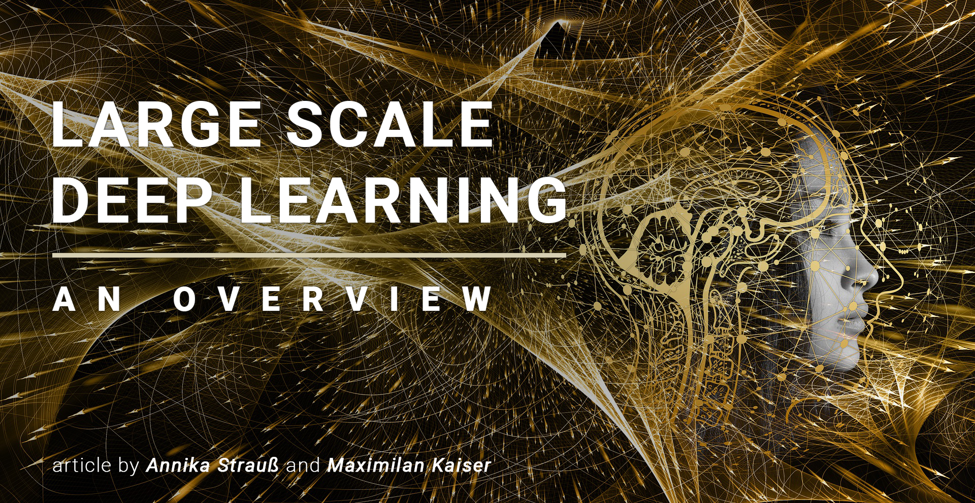
An overview of Large Scale Deep Learning

31. March 202231. March 2022 ~ mk374

article by Annika Strauß (as426) and Maximilian Kaiser (mk374)

Introduction
Improving Deep Learning with ULS for superior model training
Improving ULS and its components with the aid of Deep Learning
Outlook
Sources

1. Introduction

One of the main reasons why machine learning did not take off in the 1990s was that the lack of computational power and the size of data sets, available at that time

Since then, a lot has changed and machine learning methods have found their way into the field of ultra large systems (ULS) like f.e. Google, where they have been used very successfully for quite some time.

Two main areas of application can be distinguished:

Learn better ML models faster with very large data sets and very high computing power by parallelizing and distributing different components of the ML computation.
Deep Learning methods are developed, trained and applied to control, understand, improve and optimize specific areas within a ULS, e.g. replace multiple overcomplicated subcomponents with a single, machine learned model that still does the same job

Continue reading →

How to Scale: Real-time Tweet Delivery Architecture at Twitter

10. March 202116. March 2021 ~ Tamara Hezel

There is a lot to say about Twitters infrastructure, storage and design decisions. Starting as a Ruby-on-Rails website Twitter has grown significantly over the years. With 145 million monetizable daily users (Q3 2019), 500 million tweets (2014) and almost 40 billion US dollar market capitalization (Q4 2020) Twitter is clearly high scale. The microblogging platform, publicly launched in July 2006, is one of the biggest players in the game nowadays. But what’s the secret handling 300K QPS (queries per second) and provide a real-time tweet delivery? Read about how Redis Clusters and Tweet Fanouts revolutionized the user’s home timeline.

Continue reading →

Queueing Theory and Practice – OR: Crash Course in Queueing

11. March 20193. April 2019 ~ Alexander Georgescu

What this blog entry is about

The entry bases on the paper “The Essential Guide to Queueing Theory” written by Baron Schwartz at the company VividCortex which develops database monitoring tools.
The paper provides a somewhat opinion-oriented overview on Queueing Theory in a relatively well understandable design. It tries to make many relations to every day situations where queueing is applied and then provides a couple of annotation methods and formulas as a first approach to actual calculations.
This blog entry forms a summary of that paper but focuses on queueing in the context of ultra large scale web services and adds examples and information from my own knowledge and trivial research.

The goal of this blog entry is to provide fellow computer science and media programmers who consider working in the field of web servers an overview about queueing that might be helpful at some point to understand and maybe even make infrastructure- and design-decisions for large scale systems.

Note that some annotations do not match exactly to the paper from Schwartz because there seems to be no consensus between it and other sources either. Instead the best fitting variants have been chosen to fit this summary.

Queueing and intuitition

The paper sums up the issue as “Queueing is based on probability. […] Nothing leads you astray faster than trusting your intuition about probability. If your intuition worked, casinos would all go out of business, and your insurance rates would seem reasonable.”
Due to the skills required for survival in prehistoric times as well as due to most impressions we make nowadays in everyday life, the human mind is best suited for linear thinking. For example the Neanderthal knew that if he gathers twice as many edible fruits, he will eat off them twice as long (just imagine yourself today with snacks in the supermarket : ) ).

An exception to this is movement prediction where we know intuitively that a thrown object will fly a parabolic path. This part already comes to a limit though when we think for example of the famous “curved free kick” (Keyword: Magnus effect).
However when we try to think theoretically about things in our mind alone, we tend to resort solely to linear proportions between two values.

As we will see and calculate later, in queueing theory, relations are not just parabolic but unpredictably non-linear. A value can grow steadily for a long while until reaching a certain point and then leap rapidly towards infinity.
Let’s look at an example: You have a small web-server providing a website that allows the user to search and display images from a database.

Depending on how broad the search is, preparing and sending the search-results to the user takes a random amount between one and 3 seconds – on average that means 2 seconds. Also on average you expect 25 customers per minute.
Now the question is, how long will the user have to wait on average?

Intuitively (at least if you would not be a software dev ; ) ) you might say: Barely over two seconds. After all, handling 25 requests of 2s average each, requires just 50 seconds and thus only 5/6 (83.3%) of the systems time.
Unfortunately the reality would be a website with 5 seconds of wait time on average and far higher outliers.

The reasons are that with random request processing duration as well as random arrival time, request will naturally overlap and waiting time is automatically wasted. Whenever the server has no request to handle, those seconds are entirely lost. When multiple requests occur simultaneously later, it is not possible to “use up” that spare idle time from earlier. Instead time continues to flow and the requests have to be enqueued and wait.

The following graph shows the relation between “Residence Time” which is the whole time between arriving with a request and leaving with it (aka the site loading time) and “Utilization” of the server.

“Hockey Stick Graph” visualizing the relation between residence time and server utilization

We see a non-linear graph that is sometimes called “hockey stick graph” due to its markant shape. It shows well how the tipping point is somewhere around 80%. Past this amount of utilization, average wait time skyrockets.

The Residence Time and Utilization are only two of several values that we need to define to be able to talk on a common ground about queueing theory.

The common ground

To form a base of words and abbreviation see the following table.

Metric	Unit	Symbol	Description
Arrival Rate	Requests per time	A	The frequency of new requests to the system.
Queue Length	Waiting requests	Q	How many requests are waiting in a queue on average.
Requests (in concurrency)	Requests	R	Total requests currently waiting or being serviced.
Wait time	Time	W	Time requests spend waiting in a queue
Service time	Time	St	Time a request needs to be serviced on average. For example how long it takes to assemble the website data.
Residence time (latency)	Time	Rt	Total time from placing the request and returning the output. If ignoring data transfer delays, this naturally is W + St.
Utilization	Fraction	U	Percentage of utilization of the servers. Refers to the quote of busy-time from the total time. It’s reciprocal is the idle-time.

Basic formulas

Many of the parameters listed above are related to each other through a handful of basic formulas that are mostly trivial once you understand them.
The first and most common one is referred to “Little’s Law” as it has been formulated and proved in 1961 by John D.C. Little:

R = A * Rt

Where R is the number of total requests in the system (in queue and currently serviced), A the arrival rate and Rt the total time of a request from arrival to having been serviced.
The relation is fairly straight forward as it simply says, the longer requests take in the system and the more often they occur, the more requests will accumulate in the system.
This relationship can be resolved for the queue length as well:

Q = A * W -> Queue length = arrival rate * wait-time in queue

Another important formula is the Utilization Law:

U = A * St -> Utilization = arrival rate * service time of a request

Logical; the more services arrive and the longer time they need to be serviced, the higher utilization will be on average. To calculate this for multiple servers, just divide the utilization by servers. Of course this is for the theoretical approach only as real web servers will inevitably have an overhead through load balancing.

Last we have another important formula that says that the residence time Rt which is the latency of a request, is equal to the service time divided through the idling-percentage of the servers (1 – utilization).

Rt = St / (1-U)

Those formulas however do not allow you to predict much of how a real system will behave yet because they require you to know at least one crucial thing like average queue length, wait time in queue or the utilization.
To compute any of those, a more advanced set of formulas are needed. However before we can calculate something for a system, we first need to decide how to describe such a system.

Kendall’s annotation

A way to fulfill exactly that and describe approximately how a service system has been designed, is the “Kendall’s annotation”. It allows to differ between systems by major parameters.
Up to six parameters, each anotated by a letter, are separated by dashes:

A/T/S/P/R/D

Unfortunately the exact letters for every parameter differ a lot between sources. Therefore this blog entry describes a variant that appeared senseful to the author. Most sources use exactly the same order of parameters though.
Of all parameters, the first three are most significant as the others can be their default values for many systems.

A

The first parameter describes with what behavior the service-requests arrive. Most commonly that is one of the following letters:

M or G: Memoryless or General; means the requests occur randomly (there’s no memory of the last request). This results in an exponential distribution.
Mx: Random occurence of x requests at once.
D: Degenerate distribution; A deterministic or fixed time between requests
Ek: Erlang Distribution; Erlang Distribution with k as the shape

T

T describes the service time distribution. The same letters as for (A) are common.

S

S describes the number of services that serve requests in parallel.

P

P denotes the number of places in the system including services and queues. When this limit is reached, new requests are denied.
If omitted, this parameter is ‘infinite’ (INF).

R

R is the number of possible requesters. This is only relevant if the number of requesters is relatively low because if a significant fraction is already in queues, new requests naturally become more scarce.
If omitted, this parameter is ‘infinite’ (INF).

D

D describes the de-queueing behavior. The following abbreviations are common:

FIFO: First in first out
LIFO: Last in first out
SIRO: Service in random order
PNPN: Service order based on a priority value for every request

If omitted, this parameter is ‘FIFO’ by default.

Example

Following the Kendall’s annotation, a possible variant of a web service system is:

M/M/(s)/(b)/INF/FIFO

Where (s) is the number of requests that can be processed in parallel and (b) is the number of places for requests in memory in total.
A service system described like that means it expects requests at random intervals* and each requiring random time to process. It expects an infinite number of potential requesters because even for the largest system it is not feasible to be able to handle a significant fraction of all people with internet access at the same time**. It utilizes FIFO queues.

* Of course a system can make predictions like higher demand on certain times on the day, but that is not immediate enough because it is not a correlation between two requests. However for some types of sites (like social media for example) it can be assumed that after a user has accessed the first time, subsequent requests will occur as he keeps using the site. This type of behavior cannot be modelled with Kendall’s annotation.

** However for services available only to special, registered users the number may be limited.

Predicting the Behavior of single-server designs

A major point about those relatively theoretical approaches at queueing systems are the possibility to make certain predictions about their behavior in practice. The two numbers of interest are queue length and wait time.

In the context of the service of a large scale system, the queue length is relevant to determine the required memory for the system (or every particular machine).
The wait time on the other hand is significant for the user’s satisfaction with the whole service.
Indirectly the results of those predictions determine the required performance of the system to avoid an utilization that results in high waiting times (both tending towards infinity) as seen in the “hockey stick graph” earlier and usually in high queue lengths as well.

First it makes sense to look at the formula generating said graph for a queue that has the Kendall annotation M/M/1. That means it has random request- and service time, infinite requesters and queue-memmory and unitlizes a FIFO principle. That all runs on a single server.
The formula is:

R = S / (1 – U)

Where R is the total wait time (“residence time”), S the service time and U the utilization of the server.
Following this, the residence time is proportional to 1/(1-U). That’s often referred to as the stretch factor because it describes how much the real total wait time is stretched compared to the time needed to process a request after it left the queue.

Try out the formula here with this interactive online tool (U has been used as x and R as y).
You will notice that the lower S is, the more the critical percentage of utilization can be put off. As a rule of thumb the following can be deduced: Halving the idle capacity, doubles the whole, average response time!

Using the graph formula together with “Little’s Law” mentioned earlier, it is possible to compute further values related to the queue:

R = U / (1-U)

Where R is the average number of customers currently in the system (in queue and currently serviced).

Q = U² / (1 – U)

Where Q is the average queue length.

Eventually the time W requests wait in a queue before being serviced can be computed on average as:

W = U*St / (1-U)

Where St the service time and U the utilization of the server.

Predicting the behavior of multi-server designs

The “correct method”: The Erlang formulas

Agner Erlang who pioneered in the field of telecommunications formulated a series of equations in his field. For example one to predict how many telephone lines would be needed to carry an expected volume of calls.
A modern form of the formula involves the unit nowadays known as “Erlang” that describes the service demand. Indirectly the amount of Erlang is equal to the amount of concurrency in the optimal case and therefore the number of servers required to handle all requests.

A practical example are the backbone-telephone lines. Naturally one telephone line can “service” 60 minutes of talk in one hour. That results in exactly 1 Erlang.
Now if the real requests sum up to 600 1-minute calls in one hour, that results in 600 minutes of talk and therefore 10 Erlangs.
In practice of course a backbone with 10 lines and said demand would mean that calls would often need to wait for a free line.

This is where Erlang’s formula ‘C’ comes into play:

ErlangC where A is the request load in Erlangs and M is the number of servers.

This massive, internally iterative formula calculates the probability that a new request has no free line and therefore has to wait in a queue.
A is the request load (the current demand) in Erlangs and M is the number of total servers (or telephone lines in this example).

Wolfram Alpha allows to see this formula in action.

As expected, for the edge-case of 10 Erlang of demand and 10 available servers, the probability that the new request has to wait is practically 100% because the probability that all calls coincidentally line up accurately one after another is negligible low.
With 11 servers or telephone lines that result in a system that allows more overlapping, the result of the Erlang C formula is already about 68%.

Applying “Little’s Law” it is again possible to derive different formulas to compute desired values, however Erlang’s formulas are not easy to apply and very unintuitive. For this reason, an approximation has been found.

The aproximated method

For the case that there is one waiting queue but Xs servers, a modification of the earlier basic formula can be used:

Rt = St / (1-U^Xs)

Where S is still the service time and U the utilization.
By applying the number of servers as an exponent to the utilization, the formula is equal to the old formula in the case of 1 server. Furthermore for other cases it results only in an underestimation of total request time of up to 10%. More information can be found in Cpt 2 of “Analyzing Computer System Performance With Perl::PDQ (Springer, 2005)” by Neil Gunther.

One common queue or one queue per server?

Using the formulas, the answer to this question is always that a single queue is more efficient. The logical reason becomes clear if we keep in mind that processing requests also takes random amount of time. This can result in a situation where one server is occupied with a large request while the other server has handled its whole queue already and now has to idle.
This is why server infrastructure tends to use “load balancers” that maintain a queue of user requests and spreads them to servers.
However because transmitting requests from the balancer to a server is taking time too, the servers usually hold queues themselves to ensure to be able to work constantly.

Nevertheless, sophisticated algorithms are required for load balancers to ensure a stable system especially under unusually high load or when servers drop out. This topic is handled in other blog entries.

You can experiment with the Erlang C formula modified to compute the residence time depending on the number of servers here.
This shows how a higher number of servers also allows for better utilization of the whole system before the wait time rises too much.

Problems and Limitations

Certain precautions have to be taken before the computations above can be used in a reliable way.

Exact measurements

The two key values of the system, service time S and current utilization U need to be known accurately. This can be tricky in server environments where random network- and infrastructure-delays are added under certain circumstances or where servicing can require waiting on other, secondary services (common nowadays when building serverless websites).
A quality measure of modern server management systems are the ability to determine this and especially the utilization of the system.

Ensuring exponential distribution

While this is typical, it has to be ensured that service times do spread sufficiently close to an exponential distribution.

Cross-dependency

Modern websites are often built “serverless” and require assembling data from different sources. It is possible to assume an abstraction and only view the desired layer of services (like only the outer that delivers to the users, or for example the system inside that delivers only the images to the other process that assemble the website). However things become less predictable when a sub-service utilizes a resource that is currently needed by a different request.

Conclusions

Due to those reasons, the authors of the major paper this blog entry is based on, suggest that the queueing theory described above is most suited for everyday and physical problems. There they can be applied for relatively simple decisions. Additionally they can be used to find possible problem-causes when an actual system does not behave as assumed. In the end they mainly help to adjust peoples personal intuition that often is wrong due to the non-linearity of relations in queueing problems.

Personally I find that knowing about queueing theory and having experimented with the formulas can indeed open ones eyes to what is actually predictable and what is not. Furthermore together with modern observation tools for server systems, I would definitely suggest trying to apply the concepts and formulas to verify whether a certain system is working in an optimal way or not. Last but not least they can form a starting point when beginning to design a server infrastructure.