
In the course of attending the lecture “Ultra Large Scale Systems” I was intrigued by the subject of traffic load balancing in ultra-large-scale systems. Out of this large topic I decided to look at traffic distribution at the frontend in detail and held a presentation about it as part of this lecture. As this subject has proven to be difficult to comprehend, as long as all related factors are considered, multiple questions remained open. In order to elaborate on these questions I decided to write this blog post to provide a more detailed view of this topic for those interested. Herein, I will not discuss the subject of traffic load balancing inside an internal infrastructure, however corresponding literature can be found at the end of this article. Despite concentrating only on the frontend part of the equation an in-depth look into the workings of traffic load balancing will be provided.
Historically grown structures of the internet
The “internet” started somewhere in late 1969 as the so-called ARPANET. In those days, it was exclusively used by scientists to connect their mainframe computers. These in turn were interconnected among each other by Interface Message Processors (IMP), a predecessor of modern routers, which enables network communication through packet switching. However, the underlying protocols were fairly unreliable in heterogeneous environments, because they were specifically designed for a certain transmission medium. In 1974 Vinton Cerf and Robert Kahn, commonly known as the “fathers of the internet”, published their research paper entitled “A Protocol for Packet Network Intercommunication”. The objective of this work was to find a proper solution for connecting such diverse networks and their findings provided the base for the internet protocol suite TCP/IP in the following years. The subsequent migration of the entire ARPANET to these protocols was finally completed in early 1983 and took around six months according to Robert Kahn. At this time the term “internet” slowly began to spread around the world. In addition to this, the Domain Name System (DNS) protocol was developed in 1984. From now on it was possible to address computers in a more native way by using human-readable names instead of IP addresses. Today, all these protocols create the foundation for most connections on the internet.
Generally speaking, today’s internet giants like e.g. Google, Facebook or Dropbox are still based on these previous developments in how they deliver data to their users. In relation to the past, due to the massive increase in scale of dimensions, completely new thoughts and strategies are now necessary in order to meet the requirements. The desire for a change of the existing protocols is great, but if you consider that just the migration of the ARPANET with a significantly lower number of computers connected took six months, then such a fundamental change with several billion devices is quiet hard to imagine. In the old days, often a single web server was sufficient for all your user needs. You can simply assign an IP address to your web server, associate it with a DNS record and advertise its IP address via the core internet routing protocol BGP. In most cases, you don’t have to worry about scalability or high availability and you rely only on the BGP, which takes care of a generic load distribution across redundant network paths and increases the availability of your web server automatically by routing around unavailable infrastructure.
Bigger does not automatically mean better
Today, if you were in the role of an ultra-large-scale system operator such as Dropbox you have to handle roughly half a billion users, who meanwhile stored an exabyte of data. On the network layer this means many millions of requests every second and implies terabits of traffic. As you may have already guessed, this huge demand could certainly not be managed by a single web server. Even if you did have a supercomputer that was able to handle all these requests in some way, it is not recommended to pursue a strategy that relies upon a single point of failure. For the sake of argument, let’s assume you have this unbelievably powerful machine, which is connected to a network that never fails. At this point, please remember the 8 fallacies of distributed computing, which point out that this is only an idealized scenario and will probably never become reality. However, would that configuration be able to meet your needs as the operator? The answer is definitely no. Even such a configuration would still be limited by the physical constraints of the network layer. For instance, the speed of light is a fundamental physical constant that limits the transfer speed for fiber optic cables. This results in an upper boundary on how fast data can be served depending upon the distance it has to travel. Thus, even in an ideal world one thing is absolutely sure: When you’re operating in the context of ultra-large-scale systems, putting all your eggs in one basket is a recipe for total disaster, in other words a single point of failure is always the worst idea.
As already indicated, all the internet giants of today have thousands and thousands of machines and even more users, many of whom issue multiple requests at a time. The keyword to face this challenge is called “traffic load balancing”. This describes the approach for deciding which of the many machines in your datacenters will serve a particular request. Ideally, the overall traffic is distributed across multiple nodes, datacenters and machines in an “optimal” way. But what does the term “optimal” mean in this context? Unfortunately, there’s no definite answer, because the optimal solution depends on various factors, such as:
- The hierarchical level for evaluating the problem or in other words does the problem exists either inside (local) or outside (global) your datacenter.
- The technical level for evaluating the problem, which means – is it more likely a hardware or a software issue.
- The basic type of the traffic you’re dealing with.
Let’s pretend to take the role of the ultra-large-scale system operator Facebook and start by reviewing two typical traffic scenarios: A search request for a mates profile and an upload request for a short video of your cat doing crazy stuff. In the first case, users expect that their search query will be processed in a short time and they get their results quickly. That’s why for a search request the most important variable is latency. In the other case, users expect that their video upload takes a certain amount of time, but also look for that their request will succeed the first time. Therefore, the most important variable for a video upload is throughput. These differing needs of the two requests are crucial to determine the optimal distribution for each request at the global level:
- The search request should preferably be sent to our nearest datacenter, which could be estimated by the aid of the round-trip time (RTT), because our purpose is to minimize the latency on the request.
- By contrast, the video upload stream will be routed on a different network path and ideally to a node that is currently underutilized, because our focus is now on maximizing the throughput rather than latency.
On the local level in turn it is often assumed that all our machines within the datacenter are at equal distance to the user and connected to the same network. Therefore, an optimal load distribution follows in the first place a balanced utilization of the resources and protects a single web server from overloading.
There is no doubt, that the above example only depicts a quiet simplified scenario. Under real conditions many more factors have been taken into consideration for an optimal load distribution. For instance, in certain cases it is much more important to direct requests to a datacenter for keeping the caches warm while the datacenter itself is slightly farther away. Another example would be the avoidance of network congestions through routing non-interactive traffic to a datacenter in a completely different region. Traffic load balancing, especially for ultra-large-scale systems operators, is anything but easy to realize and needs to be permanently refined. Typically, the search for an optimal load distribution is taking place at multiple levels, which will be described in the following sections. For the sake of accuracy, it is considered that HTTP requests will be sent over TCP. Traffic load balancing of stateless services such as DNS over UDP is minimally different, but most of the principles that will be described are usually applicable in case of stateless services as well.
First step in the right direction is called “Edge”
To meet the requirements caused by the massive increase in scale of dimensions, effectively all of today’s internet giants have built up an extensive network of points of presence (PoPs) spread around the world named “Edge”. By definition, a PoP is a node within a communication system that establishes connections between two or more networks. A well-known example is the internet PoP, which is the local access point that allows users to connect to the wide area network of their internet service provider (ISP). In our context, Edge takes advantage of this principle: The most of you may be familiar with the basic idea of content delivery networks (CDN), terminating TCP connections close to the user, which results in an improved user experience because of extremely reduced latencies. By way of illustration using the example of Dropbox, you’ll now see a comparison of an HTTP request latency made directly to a datacenter and the same request made through a PoP:
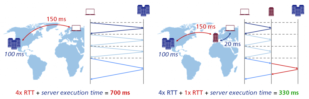
As it can be seen, in case of a direct connection between the user in Europe and our datacenter in the USA the round-trip time (RTT) is significantly higher compared to establishing the connection using a PoP. This means that by putting the PoP close to the user, it is possible to improve latency by more than factor of two!
Minimized network congestion as a positive side effect
In addition, the users benefit from faster file uploads and downloads, because latency may also cause network congestion due to long-distance transmission paths. Just as a reminder, the congestion window (CWND) is a TCP state variable that limits the amount of data which can be send into the network before receiving an acknowledgement (ACK). The receiver window (RWND) in turn is a variable which advertises the amount of data that the destination can receive. Together, both of them are used to regulate the data flow within TCP connections to minimize congestion and improve network performance. Commonly, network congestion occurs when packets sent from a source exceed what the destination can handle. If the buffers at the destination get filled up, packets are temporarily stored at both ends of the connection as they wait to be forwarded to the upper layers. This often leads to network congestion associated with packet loss, retransmissions, reduced data throughput, performance degradation and in worst case the network may even collapse. During the so called “slow start”, which is a part of the congestion control strategy used by TCP, the CWND size is increased exponentially to reach the maximum transfer rate as fast as possible. It increases as long as TCP confirms that the network is able to transmit the data without errors. Nevertheless, this procedure is only repeated until the maximum advertised window (RWND) is reached. Subsequently, the so called “congestion avoidance” takes place and continues to increase the CWND as long as no errors occur. This means that the transfer rate in a TCP connection, determined by the rate of incoming ACK, depends on the bottleneck in the round-trip time (RTT) between sender and receiver. However, the adaptive CWND size allows TCP to be flexible enough to deal with arising network congestion, because the path to the destination was permanently analyzed beforehand. It can adjust the CWND for reaching an optimal transfer rate with minimal packet loss.
Let’s keep that in mind and take up again our initial thought to see how latency affects growth of the CWND during file uploads:
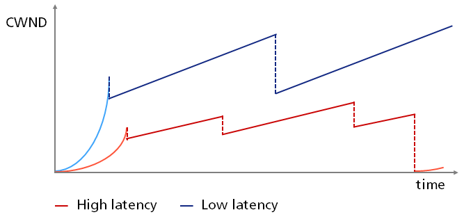
By using the example of Dropbox, you can see the impacts arising from low latency compared to high latency for connections with or without a PoP respectively. The transfer history of our client with lower latency is progressing through the so called “slow start” more quickly, because as you already know this procedure is depending on the RTT. This client also settles down on a higher threshold for the so called “congestion avoidance”, because its connections have a lower level of packet loss. This is due to the fact that packets spend less time on the internet and its possibly congested nodes. Once they reach the PoP, you can take them into our own network.
Enhanced approach for congestion avoidance
As you may have already guessed the congestion control strategy as described above is no longer an adequate response due to the transfer speeds that are available today. Since late 1980 the internet has managed network congestion through indications of packet loss to reduce the transfer rate. This worked well for many years, because the small buffers of the nodes were well aligned to the overall low bandwidth of the internet. As a result, the buffers get filled up and drop packets that they could not handle anymore at the right time when the sender has begun transmitting data too fast.
In today’s diverse networks the previous strategy for congestion control is slightly problematic. Therefore, in small buffers on the one hand, packet loss often occurs before congestion. Through commodity switches having such small buffers, which are used in combination with today’s high transfer speeds, the congestion control strategy based on packet loss can result in extremely bad throughput because it commonly overreacts. The consequence is a decreased sending rate upon packet loss that is even caused by temporary traffic bursts. In large buffers on the other hand, congestion occurs usually before packet loss. At the Edge of today’s internet, the congestion control strategy based on packet loss causes the so called “bufferbloat” problem, by repeatedly filling these large buffers in many nodes on the last mile which results in an useless queuing delay.
That’s why going forward a new congestion control strategy, which responds to actual congestion rather than packet loss, is much-needed. The Bottleneck Bandwidth and Round-trip propagation time (BBR) developed by Google tackles this with a total rewrite of congestion control. They started from scratch by using a completely new paradigm: For the decision on how fast data can be send over the network, BBR considers how fast the network is delivering the data. For that to happen, it uses recent measurement of the network’s transmission rate and round-trip time (RTT) to generate a model that includes the current maximum bandwidth that is available as well as its minimum current round-trip delay. Afterwards, this model is used by BBR to control both how fast data is transmitted and the maximum amount of data that is possible in the network at any time.
How to detect the optimal PoP locations
After our extensive discursion on network congestion and how it may be avoided, let’s get back to Edge and its network of PoPs. In case of Dropbox, according to the latest information, they have roughly 20 PoP spread across the world. This year it is planned to increase their network by examining the feasibility of further PoPs in Latin America, Middle East and the Asia-Pacific region. Unfortunately, the procedure for selecting PoP locations, which was easy first, now becomes more and more complicated. Besides focusing on available backbone capacity, peering connectivity and submarine cables, all the existing locations have to be considered too.
Their method to select PoPs is still done manually but is already assisted by algorithms. Even with a small number of PoPs and without assistive software it is challenging to choose between, for instance a PoP in Latin America or Australia. Regardless of the number of PoPs, the basic question always remains: What location will benefit the users better? For this purpose, the following short “brute-force” approach helps them to solve the problem:
- First, the Earth is divided into multiple levels of so called “S2 regions”, which are based on the S2 Geometry library provided by Google. Through this, it is possible to project all your data in a three-dimensional space instead of a two-dimensional projection what results a more detailed view of the Earth.
- Then all existing PoPs are assigned accordingly to the prior generated map.
- Afterwards, the distance to nearest PoP for all regions weighted by “population” is determined. In this context the term “population” refers to something like the total number of people in a specific area as well as the number of existing or potential users. This is used for optimization purposes.
- Now, exhaustive search is done to find the “optimal” location for the PoP. In connection with that, L1 or L2 loss functions are used to minimize the error for determining the score of each placement. Hence, they try to compensate internet quirks such as the effects of latency on the throughput of TCP connections.
- Finally, the new-found location will be added to the map as well.
- The steps 3 to 5 are repeated for all PoPs until an “optimal” location is found for each of them.
The attentive reader may have already seen that the above problem can also be solved by more sophisticated methods like Gradient Descent or Bayesian Optimization. This is indeed true, but the problem space is relatively small with roughly 100.000 S2 regions, so that they can just brute-force through it and still achieve a satisfying result instead of running the risk to get stuck on a local optimum.
The beating heart of the Edge
Now, let’s have a closer look at Global Server Load Balancing (GSLB), which is completely without doubt the most important part of the Edge. It is responsible for load distribution of the users across all PoPs. This usually means that a user is sent to the closest PoP, which has free capacity and is not under maintenance. Calling the GSLB the “most important part” here is due to the fact that if it misroutes users to a suboptimal PoP frequently, then it potentially reduces performance and your Edge may be rendered useless. Using the example of Dropbox, commonly used techniques for GSLB should be discussed hereinafter by showing up the pros and cons.
Keep things easy with BGP anycast
Anycast is by far the easiest method to implement traffic load balancing, because it completely relies on the Border Gateway Protocol (BGP). Just as a quick reminder, anycast is a basic routing scheme where the group members are addressed by a so called “one-to-one-of-many” association. This means that packets are routed to any single member belonging to a group of potential receivers, which are all identified by the same destination IP address. The routing algorithm then selects a single receiver from the group based on a metric that relies on the least number of hops. This leads to the fact that packets are always routed to the topologically nearest member of an anycast group.
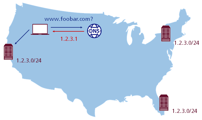
As it can be seen, to use anycast it is sufficient to just start advertising the same IP subnet from all PoPs and the internet respectively. DNS will deliver packets to the “optimal” location as if by magic. Even though you get a rudimentary failover mechanism for free and the setup is quiet simple, anycast has a lot of drawbacks, so let’s have a look at these in detail.
Anycast is not the silver bullet
Above, it was mentioned that BGP automatically selects the “optimal” route to a PoP and from a general point of view this is not incorrect. However, the policy of Dropbox favors network paths that are likely to optimize the traffic performance. But the BGP does not know anything about latency, throughput or packet loss and it relies only on attributes such as path length, which turns out as inadequate heuristics for proximity and performance. Thus, traffic load balancing based on anycast is optimal in most cases, but it would seem that there is a poor behavior on high percentiles if there is only a small or medium number of PoPs involved. However, it looms that the probability of routing users to the wrong destination in networks using anycast decreases with the number of PoPs. Nevertheless, it is possible that with an increasing number of PoPs, anycast may eventually exceed the traffic load balancing method based on DNS, which is discussed below.
Limited traffic steering capabilities
Basically, with anycast control over the traffic is very limited, so that the capacity of a node may not be able to forward all traffic you would like to send over it. Considering that peering capacity is quiet limited, rapid growth in demand can quickly result in an overstrain of the capacity of an existing interconnection. Short-time peaks in demand due to an event or a holiday as well as reductions in capacity caused by failures can lead to variations in demand and available capacity. In any of these cases the decisions BGP makes won’t be affected by surrounding factors, as it is not aware of capacity problems and related conflicts. Nevertheless, you can do some “lightweight” traffic distribution using specific parameters of BGP in the announcements or by explicitly communicating with other providers to establish a peering connection, but all this is not scalable at all. Another pitfall of anycast is that careful drain of PoPs at times of reduced demand is effectively impossible, since BGP balances packets, not connections. As soon as the routing table changes, all incoming TCP connections will immediately be routed to the next best PoP and the user’s request will be refused by a reset (RST).
The crux of the matter is often hard to find
Most commonly, general conclusions about traffic distribution with anycast are not trivial, since it involves the state of internet routing at a given moment. Troubleshooting performance issues with anycast is like looking for a needle in a haystack and usually requires a lot of traceroutes as well as a long wind in communicating with involved providers. It is worth mentioning again, that in the case of draining PoPs, any connectivity change in the internet has a possibility to break existing TCP connections to IP addresses using anycast. Therefore, it can be quiet challenging to troubleshoot such intermittent connection issues due to routing changes and faulty or rather misconfigured hardware components.
Light and shadow of load distribution with DNS
Usually, before a client can send an HTTP request, it often has to look up an IP address first using DNS. This provides the perfect opportunity for introducing our next common method to manage traffic distribution called DNS load balancing. The simplest way here is to return multiple A records for IPv4 and AAAA records for IPv6 respectively in the DNS reply and let the client select an IP address randomly. While the basic idea is quiet simple and easy to implement, it still has multiple challenges.
The first problem is that you have only little control over the client behavior, because records are selected arbitrary and each will attract roughly the same amount of traffic. But is there any way to minimize this problem? On paper, you could use a SRV record to predefine specific priorities, but unfortunately these records have not yet been adopted for HTTP.
Our next potential problem is due to the fact that usually the client cannot determine the closest IP address. You can bypass this obstacle by using an anycast IP address for authoritative name servers and take advantage of the fact that DNS queries will lead to the nearest IP address. Thus, the server can reply addresses pointing to the closest datacenter. An improvement of that builds a map of all networks as well as their approximate geographical locations and serves corresponding DNS replies. However, this approach implies a much more complex DNS server implementation and a maintaining effort to keep the location mapping up to date.
The devil is often in the detail
Of course, none of the solutions above are easy to realize, because of fundamental characteristics of DNS: A user rarely queries authoritative name servers directly. Instead, a recursive DNS server is usually located between a user and the name server. This server proxies queries of the users and often provides a caching layer. Thereby, the DNS middleman has the following three implications on traffic management:
- Recursive resolution of IP addresses
- Multiple nondeterministic reply network paths
- Additional caching problems
As you may have already guessed the recursive resolution of IP addresses is quiet problematic, because instead of the user’s IP address an authoritative name server sees the IP address of the recursive resolver. This is a huge limitation, as it only allows replies optimized for the shortest distance between the location of the resolver and the name server. To tackle this issue, you can use the so called “EDNS0” extension, which includes information about the IP subnet of the client inside the DNS query sent by a recursive resolver. This way, an authoritative name server returns a response that is optimal from the perspective of the user. Although this is not yet standard, the biggest DNS resolvers such as Google have decided to support it already.
The difficulty here is not only to return the optimal IP address by a name server for a given user’s request, but that name server may be responsible for serving thousands or even millions of users spread across multiple regions. For example, a large nationwide ISP might operate name servers for its entire network inside one datacenter, which has interconnections for each provided area. These name servers would always return the IP address that is optimal from the perspective of the ISP, despite there being better network paths for their users. But what does the term “optimal” mean in the context of DNS load balancing? The most obvious answer to this question is a location that is closest to the user. However, there are existing additional criteria. First of all, the DNS load balancer has to ensure that the selected datacenter and its network are working properly, because sending user requests to a datacenter that has currently problems would be a bad idea. Thus, it is essential to integrate the authoritative DNS server into the infrastructure monitoring.
The last implication of the DNS middleman is related to caching. Due to the fact that authoritative name servers cannot flush the caches of a resolver remotely, it is best practice to assign a relatively low time to live (TTL) for DNS records. This effectively sets a lower boundary on how quickly DNS changes can be theoretically propagated to users. But the value has to be set very carefully, since if the TTL is too short, it results in a higher load on your DNS servers plus an increased latency, because clients have to perform DNS queries more often. Moreover, Dropbox concluded that the TTL value in DNS records is fairly unreliable. They used a TTL of one minute for their top level domain (TLD) and in case of changes it takes about 15 minutes to drain 90% of the traffic and in total roughly a full hour to drain additional 5% of traffic.
DNS load balancing in the field
Despite all of the problems that are shown above, DNS is still a very effective way for traffic load balancing in ultra-large-scale systems.
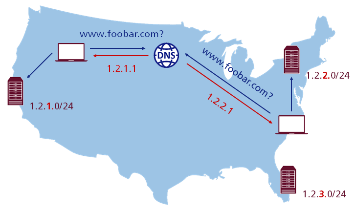
By using the example of Dropbox, you can see an approach where each PoP has its own unique unicast IP address space and DNS is responsible for assigning different IP addresses to the users based on their geographical location. Just as a quick reminder, unicast is another basic routing scheme where sender and receiver are addressed by a so called “one-to-one” association. This means that each destination IP address uniquely identifies a single receiver. It gives them control over traffic distribution and also allows a careful drain of PoPs. It is worth mentioning that conclusions in the context of a unicast setup are much easier and troubleshooting becomes simpler as well.
Hybrid unicast/anycast combines the best of both worlds
Finally, let’s briefly cover one of the composite approaches to GSLB, which is a hybrid setup with a combination of unicast and anycast. This allows getting all benefits from unicast and the ability to quickly drain PoPs if it is required along with DNS replies corresponding to geographical locations.
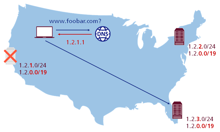
As it can be seen, this approach is used by Dropbox to announce the unicast IP subnet of a PoP and one of its IP supernets simultaneously from all of the PoPs. However, it implies that every PoP needs a configuration that is able to handle traffic destined to any PoP. This will be realized inside a PoP by a L4 load balancer using virtual IP addresses (VIP). Basically, these VIPs are not assigned to any particular machine and usually shared across many of them. However, from the perspective of the user a VIP remains a single, regular IP address. On paper, this practice allows to hide the number of machines behind a specific VIP and other implementation details. This gives them the ability to quickly switch between unicast and anycast IP addresses as needed and also an immediate fallback without waiting for the unreliable TTL to expire. Thereby, a careful drain of PoPs is possible and all the other benefits of DNS load balancing will remain as well. All of that comes at a relatively small operational cost with a slightly more complex setup and may cause trouble in respect of scalability, once the amount of several thousand VIPs is reached. But the positive side effect of this approach is that the configuration of all PoPs becomes clearly more uniform.
Real User Measurement brings light into the darkness
At all the methods for traffic load balancing discussed up until now one critical problem always remains: None of them covers the actual performance which a user experiences. Instead, they rely only on some approximations such as the number of hops used by BGP and the assignment of IP addresses in case of DNS based on geographical location. However, this lack of knowledge can be bridged by using Real User Measurement (RUM). For example, Dropbox is collecting such detailed performance information from their desktop clients. As they said, a lot of time is put into the implementation of a measurement framework, helping them to estimate the reliability of their Edge from the perspective of a user. The basic procedure is pretty simple: From time to time, a subset of clients checks the availability of their PoPs and reports back the results. Afterwards, they extended this by collecting latency information too, which allows them a more detailed view of the internet.
Additionally, they build a separate mapping by joining data from their DNS and HTTP servers. On top of that, they added information about the IP subnet of their clients from the so called “EDNS0” extension, which is sent inside the DNS query by a recursive resolver. Now, they combined this with the aggregated latencies, BGP configuration, peering information and utilization data from the infrastructure monitoring to create a decidedly mapping of the connection between clients and their Edge. Finally, they compared this mapping to both anycast as well as the assignment of IP addresses in case of DNS based on geographical location and packed it into a so called “radix tree”, which is a special data structure for a memory-optimized prefix tree, to upload it onto a DNS server.
To expand the mapping for extrapolation purposes they made their decisions using the following patterns: In case that all samples for a node have the same “optimal” PoP in the end, they conclude that all IP address ranges announced by that node should lead to that PoP. Otherwise, if a node has multiple “optimal” PoPs, they break it down into announced IP address ranges. While doing so, for each one it is assumed that if all measurements in an IP address range end up at the same PoP, this choice can be extrapolated to the whole range as well. With this approach they are able to double their map coverage, make it more robust to changes and generate a mapping based on a smaller amount of data.
Reaching the safe haven
In conclusion, all this back and forth with finding out a user’s IP address based on its resolver, the effectiveness of assigning an IP address in case of DNS based on geographical location, the fitness of decisions made by BGP and so on are all no longer necessary after a request arrives at the Edge. Because from that moment on, you know the IP address of each user and even have a corresponding round-trip time (RTT) measurement. Now, it is possible to route users on a higher level such as embedding a link to a specific PoP in the HTML file. This allows traffic distribution on a more detailed level.
As you may have realized by reading this article, traffic load balancing is a difficult and complex problem that is really challenging, if you want to consider all related factors. In addition to the strategies described above, there are much more traffic distribution algorithms and techniques to reach high availability in ultra-large-scale systems. If you want to know more about the idea of traffic load balancing, or which facts you have to consider for developing a strategy of traffic distribution inside the PoPs, please follow the links at the end of this article.
References and further reading
- Dropbox traffic infrastructure: Edge network by Oleg Guba and Alexey Ivanov
https://blogs.dropbox.com/tech/2018/10/dropbox-traffic-infrastructure-edge-network/ - Steering oceans of content to the world by Hyojeong Kim and James Hongyi Zeng
https://code.fb.com/networking-traffic/steering-oceans-of-content-to-the-world/ - Site Reliability Engineering: Load Balancing at the Frontend by Piotr Lewandowski and Sarah Chavis
https://landing.google.com/sre/sre-book/chapters/load-balancing-frontend/ - Directing traffic: Demystifying internet-scale load balancing by Laura Nolan
https://opensource.com/article/18/10/internet-scale-load-balancing - What is CWND and RWND by Amos Ndegwa
https://blog.stackpath.com/glossary/cwnd-and-rwnd/ - TCP BBR congestion control comes to GCP – your Internet just got faster by Neal Cardwell et al.
https://cloud.google.com/blog/products/gcp/tcp-bbr-congestion-control-comes-to-gcp-your-internet-just-got-faster - What Are L1 and L2 Loss Functions? by Amit Shekhar
https://letslearnai.com/2018/03/10/what-are-l1-and-l2-loss-functions.html
Leave a Reply
You must be logged in to post a comment.