Improved Vulnerability Detection using Deep Representation Learning

Today’s software is more vulnerable to cyber attacks than ever before. The number of recorded vulnerabilities has almost constantly increased since the early 90s. The strong competition on the software market along with many innovative technologies getting released every year forces modern software companies to spend more resources on development and less resources on software quality and testing. In 2017 alone, 14.500 new vulnerabilities were recorded by the CVE (Common Vulnerability and Exposures) database, compared to the 6.000 from the previous year. This will continue in the years to come. [1]

CVE statistics — Fig. 1 – Statistics on software vulnerability reported since 1988 – *Source: NIST: US Department of Commerce* [1]

Since these problems have existed for quite some time, there are many tools that automatically uncover vulnerabilities in code bases and help the developer build better software.

Static analysers find vulnerabilities without executing the code. Dynamic analysers execute the program multiple times with different test inputs to uncover weaknesses while Symbolic execution replaces input data with symbolic values to analyse the control flow of the program. That way, every program execution path can be reproduced to uncover bugs or weaknesses. The drawback to this approach is that it is expensive to do, because it takes a lot of time. This doesn’t scale well for large code bases. [2]

All of these solutions are rule-based, which means that they can only detect a limited subset of errors. The rules have to be defined by security experts, which is a tedious and often error-prone task. To avoid these errors, multiple human experts have to be employed to define features and rules, which raises the cost of building these tools.

The advantage of Deep Learning algorithms is that they can do the feature extraction by themselves and alleviate human experts from those tasks [2]. Most importantly, they can learn vulnerability patterns on their own, provided they are fed the right training examples. In this Blog-Post, I will present a data-driven approach to solve the vulnerability detection problem with highly improved performance.

What about the data?

Every Machine Learning algorithm needs a lot of data to work properly. The first question to be answered is how finely grained does the collected data need to be. Does it suffice to only use single lines of code or functions or is it necessary to use complete classes as training data?

Granularity of the data

The approach described in VulDeePecker: A Deep Learning-Based System for Vulnerability Detection by Zhen Et al. [3] uses so-called Code Gadgets, which enable a finer granularity than the function-level approach, but still contain more information than single code lines. A Code Gadget consists of semantically related lines of code. To generate one, you have to identify a key point, the center of a vulnerability and find the semantically related lines by analysing the control flow or data flow of the program (see Fig. 2). These key points might be function calls, arrays, pointers, etc. All of the Code Gadgets in [3] were generated using library/API calls as key points. Zhen Et al. state that building a heuristic concept for mapping key points to vulnerabilities is beyond the scope of their present paper and remains to be further investigated. Additionally, Zhen Et al. focused on Buffer and resource management errors for vulnerabilities exclusively. [3]

Fig. 2 – How Code Gadgets are built by extracting a library/API function call – source: [3]

This means that their method is restricted to a specific subset of two common vulnerability types that are related to library/API calls. Any other vulnerability type or key point is not taken into account.

A broader approach is described in Automated Vulnerability Detection in Source Code Using Deep Representation Learning by Rebecca L. Russel Et al. [2]. They analyse software on the function level and don’t restrict themselves to any specific subset of vulnerability types. Instead, they leave it up to the Neural Network to find vulnerability patterns in the function code. [2]

I am going to focus on this approach, going forward.

Where to get the data from?

Since there are a lot of open-source projects, an obvious choice is to mine the needed program code from Git repositories. It is important to note that the quality of the code and the quality of the commit messages play a significant role to the overall quality of the training data. Repositories like the Linux kernel, Firefox, Thunderbird, SeaMonkey, Apache, etc. come to mind when it comes to training a vulnerability detection system for C/C++ programs. [3]

How do we label the data?

To label code vulnerabilities at a function level, there are three possibilities: using a static analyser, using a dynamic analyser and commit message tagging. Dynamic analysis takes a lot of time and is therefore impractical for labelling large amounts of data. Commit message tagging doesn’t consume much time, but produces only a small amount of high quality labels. The reason for that is that the only reliable way of finding a high quality label in a commit message is through searching for keywords like “fixed”, “buggy”, etc. and then extracting the fixed function code. This rules out most commit messages and doesn’t yield enough data points to train a model on its own.

That’s why Rebecca L. Russel Et al. [2] combined this approach with using multiple static analysers and then letting a couple of security researchers manually prune the results to exclude false positives in the labels. This resulted in two overall labels: vulnerable (1) and not vulnerable (0). [2]

Available datasets for vulnerability detection

The dataset created by Rebecca L. Russel Et al. – https://osf.io/d45bw
The labeled Code Gadgets created by Zhen Li Et al. – https://github.com/CGCL-codes/VulDeePecker
The SATE IV dataset. Contains code examples with CWE-labelled vulnerabilities [4] – https://samate.nist.gov/SATE4.html

How to build effective program representations

How can you represent a program in a form that is understood by a Neural Network? The data has to be in a numerical vector format. This means that we need to find a numerical representation of our program code that contains all of the information needed to detect vulnerabilities. This problem has been solved in Natural Language Processing (NLP) with Word Embeddings. In NLP, Vector Space Models (VSMs) are used to represent words in a $n$ -dimensional vector space where semantically similar words are located nearby each other [6]. This can be done with program code, too.

Pre-trained Word Embeddings already exist for normal NLP applications, but not for programming languages. This means that for any task in relation to classifying program code, Word Embeddings have to be trained from scratch.

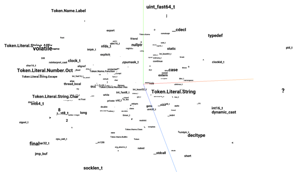
The first step is to build a vocabulary that contains all of the tokens used by the specific programming language. It makes sense to use a Lexer to build an intermediate representation of the code that uses a much smaller vocabulary size and consequently reduce the dimensionality of the training examples. That way, a lot less data is needed to train the model. All of the necessary patterns are retained in a lexed representation of the program code. An example would be the semantic meaning of string literals. Every string literal has roughly the same word embedding in the aforementioned $n$ -dimensional vector space. Replacing every string literal with a unique identifier doesn’t remove any important information from the data. For C/C++, Clang [8] is an obvious choice while a language-specific lexer has to be used for other languages. Rebecca L. Russel Et al. built their own lexer specifically for this task. [2]

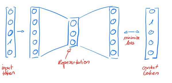
The approach for Word Embeddings used in this case is word2vec. All of the tokens from the lexed code are embedded into a $k$ -dimensional representation using a Neural Network with one hidden layer. The Neural Network is trained to predict a context token from the input token (see Fig. 3). The context size is set before training and is found by trial and error. I found that a context size of 2 performs really well. When training is finished, the hidden activations are used as Word Embeddings [6].

Fig. 3 – Neural Network used to train Word Embeddings.

The best results were achieved with a representation of size $k = 13$ and little bit of noise added to it during training to improve its resistance to overfitting [2]. The finished Embeddings look like this (see Fig. 4):

Fig. 4 – The Word Embeddings visualised in a 3-dimensional vector space. This visualisation was done using PCA for dimensionality reduction and Tensorboard for an interactive 3D plot

How do we classify our Word Embeddings?

To perform the first classification of the word vectors, CNNs are used. Their overall performance on this task is better than the performance of RNNs [2]. Additionally, you can visualise, which features they focus on for the class decision. I will refer to this point later.

The overall architecture can be described as follows: to extract the features, only one Convolutional Layer is used. This layer contains 512 filters with a filter size of $m * l$ , which means that the convolutional filters are as wide as the word embeddings. The filter height $m$ describes how many tokens are trained together at once. Consequently, the result of each convolution is a one-dimensional row vector. The ReLu activation function and a batch normalisation are applied after each convolution (see Fig. 5).

All of the inputs are restricted to a size of 500px. If an input matrix is smaller than that, it is padded with zeroes. Overall, a mini-batch size of 128 proved to give the best results.

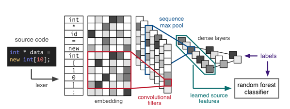
Fig. 5 – The CNN architecture used to classify the source code from functions – Source: [2]

Since the dataset is highly unbalanced with an overwhelming majority of the data being not vulnerable (0) the loss function has to weigh data points labeled as vulnerable much stronger than invulnerable ones. A surprising finding is that an ensemble classifier like a random forest performs better than the dense layers of the CNN. That way, the feature extractor of the CNN is used to extract representations that are then fed into a random forest for classification. [2]

So, how well does our new model perform?

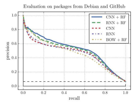
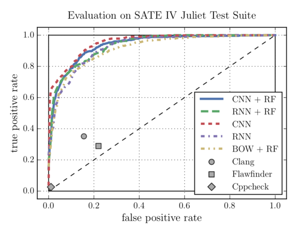
As described before, CNNs perform better than RNNs. Additionally, they have a couple of other advantages over RNNs: they train faster since their operations can be executed concurrently, they need fewer parameters to train and don’t suffer from a vanishing gradient problem. As mentioned before, the Overall best performance can be achieved with the CNN for feature extraction and a Random Forest for classification (see Fig. 6 and 7). All of the ML models by far outperform the three static analysers (see Fig. 7). [2]

Fig. 6 – recall vs. precision for vulnerability prediction on Debian and Github data – Source: [2]

Fig. 7 – False Positive rate vs. True negative rate on SATE IV Juliet Test Suite – Source: [2]

The advantage of Machine-Learning-based vulnerability detection tools is that they can analyse large code bases in a relatively short amount of time without the need to compile them first. Static analysers only return a number of vulnerabilities they found, but no posterior probability that indicates how reliable their findings are. With a Machine Learning model, a threshold can be defined, which defines how high the posterior probability needs to be for the output to be considered a relevant finding. This can be especially useful if a large code base has to be evaluated and these findings have to be reliable instead of complete. In contrast, the threshold can be lowered if the tool is used on a critical system and every possible vulnerability has to be found. The Data-Science-specific description of this is tuning the model for better recall vs. better precision.

As mentioned before, CNNs have the advantage over RNNs that the features used for classification can be visualised, so that the relevant code snippets can be highlighted. A good approach to do that is the Grad-CAM algorithm, described by Ramprasaath R. Selvaraju Et al. in [10]. RNNs don’t offer that possibility since they don’t have a sparsity constraint in their hidden layers.

The Conclusion

All of the classifiers in [2, 3, 11] perform much better on vulnerability detection tasks than the rule- or pattern-based analysers, that are used today [3]. These tools either match with a vulnerability pattern or not. They don’t return a probability of accurate their findings are. Developers have to largely prune these findings by themselves, which leads to more development time and less improvement in security since most developers aren’t security experts.

Machine Learning algorithms return findings with an posterior probability that indicates how reliable the findings are. This allows developers to instantly see, which findings have to be fixed and which findings probably are false positives. Also, the models can be tuned for better recall vs. better precision, meaning that working with a large code base, the output threshold can be raised, so that only the most relevant findings are returned. Working with critical systems, the threshold can be lowered and the findings will be more complete along with returning less relevant ones.

All of this hugely depends on the data with which the model is being trained. If the training data is of high quality, the model will perform very well. If the training data is of low quality, the model will perform very badly, independent of how advanced the model architecture is.

A model only needs to be trained once for every programming language and can then be used across many projects. Of course, these models need to be regularly fine-tuned with new vulnerabilities. But this is no huge effort and problem calls for public vulnerability datasets that are regularly updated to train ML-based vulnerability detection models. If done properly, common vulnerabilities could easily be avoided in the future.

Sources and further reading:

Is software more vulnerable today? – https://www.enisa.europa.eu/publications/info-notes/is-software-more-vulnerable-today (last access: 01.03.2019)
R. Russell et al., “Automated Vulnerability Detection in Source Code Using Deep Representation Learning,” 2018 17th IEEE International Conference on Machine Learning and Applications (ICMLA), Orlando, FL, 2018, pp. 757-762.
doi: 10.1109/ICMLA.2018.00120
Z. Li et al., “VulDeePecker: A deep learning-based system for vulnerability detection,” CoRR, vol. abs/1801.01681, 2018.
Static Analysis Tool Exposition (SATE) IV – https://samate.nist.gov/SATE4.html (last access: 01.03.2019)
Y. Zhou and A. Sharma, “Automated identification of security issues from commit messages and bug reports,” in Proc. 2017 11th Joint Meeting Foundations of Software Engineering, pp. 914–919, 2017.
Vector Representations of Words – https://www.tensorflow.org/tutorials/representation/word2vec (last access: 03.03.2019)
Learn Word2Vec by implementing it in tensorflow – https://towardsdatascience.com/learn-word2vec-by-implementing-it-in-tensorflow-45641adaf2ac (last access: 03.03.2019)
Clang: a C language family frontend for LLVM – https://clang.llvm.org/ (last access: 04.03.2019)
Basic evaluation measures from the confusion matrix – https://classeval.wordpress.com/introduction/basic-evaluation-measures/ (last access: 04.03.2019)
R. R.Selvaraju, A. Das, R. Vedantam, M. Cogswell,
D. Parikh, and D. Batra. “Grad-cam: Why did you say that?
visual explanations from deep networks via gradient-based
localization.” arXiv:1611.01646, 2016.
J. A. Harer, L. Y. Kim, R. L. Russell, O. Ozdemir, L. R. Kosta, A. Rangamani, L. H. Hamilton, G. I. Centeno, J. R. Key, P. M. Ellingwood, M. W. McConley, J. M. Opper, P. Chin, and T. Lazovich. “Automated software vulnerability detection with machine learning.” arXiv:1803.04497, February 2018