Federated Learning

The world is enriched daily with the latest and most sophisticated achievements of Artificial Intelligence (AI). But one challenge that all new technologies need to take seriously is training time. With deep neural networks and the computing power available today, it is finally possible to perform the most complex analyses without need of pre-processing and feature selection. This makes it possible to apply new models to numerous applications. The only thing needed is tons of training data, a good model and a lot of patience during training.

Continue reading

About using Machine Learning to improve performance of Go programs

Gophers

This Blogpost contains some thoughts on learning the sizes arrays, slices or maps are going to reach using Machine Learning (ML) to increase  programs’ performances by allocating the necessary memory in advance instead of reallocating every time new elements are appended.

What made me write this blogpost?

Well first of all I had to because it is part of the lecture Ultra Largescale Systems (ULS) I attended past winter term. But as an introduction I’ll tell you what made me choose this topic: I started to learn Golang and coming from mainly Java, Python and JavaScript the concept of Arrays with fixed sizes and Slices wrapped around them for convenience was new to me. When I understood that initializing them with the correct capacity is good for performance and memory usage I always tried to so. Until I came to some use case where I could not know the capacity in advance. At almost the same time we talked about “ML for Systems” in the ULS-lecture. There the power of ML is used to speed up Databases, loadbalance Elastic Search Queries and other things. So I came up with the idea of ML for programming languages in this case for learning capacities in Golang. By the way I wanted to try out ML in Go, which is said to bring some performance advantages compared to python and is easier to deliver. But neither ML in Go (go for ML) nor ML on Go is topic of this post, though both appear at some parts.

The goal in more detail

As explained in various blogposts like here and there, arrays have fixed sizes in Go. For convenient manipulation anyway they can be wrapped by slices. Thus appending to a slice that reached its capacity needs to create a new slice with a larger underling array, copy the contents of the old slice to the new one and then replace the old one by the new one. This is what the append method does. That this process is more time consuming than appending to a slice that has a sufficient capacity can be shown with some very simple code that just appends 100 times to a test slice in a loop. Once the slice is initialized with a capacity of zero and once with 100. For both cases we calculate the durations it takes and compare them. Since those durations can vary for the same kind of initialization we run this 1000 times each and calculate the average duration to get more meaningful results. The averages are calculated by the method printSummary which is left out here in order to keep track of things. However the whole code can be found on GitHub.

func main() {
times := 1000
results := make([]time.Duration, 0, times)
for t := 0; t < times; t++ {
start := time.Now()
// initialize either with capacity of 0
// test := make([]int, 0)
// or initialize with final capacity of 100
test := make([]int, 0, 100)
for i := 0; i < 100; i++ {
// uncomment to see how the capacity grows in larger steps
// fmt.Println(cap(test), len(test))
test = append(test, i)
}
elapsed := time.Now().Sub(start)
results = append(results, elapsed)
}
printSummary(results)
}

As expected the correct initialized version runs with an average of 1714ns faster than the other one with an average of 2409ns. Of course those durations are still just samples and vary if the code runs multiple times. But in over 20 runs each there is only one average value of the bad initialized slice lower than some of the good ones.

If we also take a look at the capacity the slower version ends up with, we see that this is 128 instead of the required 100. This is because append always doubles the capacity if it reaches the limit.

So we can see that it is worth setting the capacity correct in advance for performance and resource consumption reasons. But this is not always as easy as in the example we just saw and sometimes it is not even possible to know the length a slice will grow up to in advance. In those cases it might make sense to let the program learn the required capacities. It could be helpful at initialization with make as well as for growing with append.

A basic example

Setup

To check out feasibility I created a basic example that is a bit more complex than the first one but still possible to calculate as well. It iterates over index j and value s of a slice of random integer samples and for each of them the test slice is created. Then we append s times three values and one value j times. So the final length (and required capacity) of test can be calculated as s*3+j.

Also in this loop training data gets gathered. One sample consists of s and j as input and len(test) as label. Since the main goal of this scenario is to check if it’s worth using a trained ML model to predict the required capacity, this data is collected always to create equal conditions for every test case. Ways to avoid the time expensive training and data collection at runtime are discussed later.

func appendInBasicLoop(kind string) training.Examples {
samp := getSamples(1000)
data := make([]training.Example, 0, len(samp))
times := 1000
results := make([]time.Duration, 0, times)
for trys := 0; trys < times; trys++ {
start := time.Now()
for j, s := range samp {
var test []int
switch kind {
case "zero":
test = make([]int, 0)
case "calc":
test = make([]int, 0, s*3+j)
case "func":
test = make([]int, 0, getCap(s, j))
case "model":
test = make([]int, 0, getCapFromModel(s, j))
case "model+1":
test = make([]int, 0, getCapFromModel(s, j)+1)
}
for i := 0; i < s; i++ {
test = append(test, i)
test = append(test, j)
test = append(test, s)
}
for k := 0; k < j; k++ {
test = append(test, k)
}
data = append(data,
training.Example{
Input: []float64{float64(s), float64(j)},
Response: []float64{float64(len(test))}})
}
elapsed := time.Now().Sub(start)
results = append(results, elapsed)
}
printSummary(results)
return data
}

As implementation for the ML part I chose go-deep. I picked it from this list because it looked well documented, easy to use and sufficient for my needs, though not perfect.

I used the collected training data to train a MLP (Multi Layer Perceptron) with two hidden layers containing two and five neurons. Of course I configured RegressionMode to use Identity as activation function in the output layer and MSE (Mean Square Error) as loss function. I also played around with some other hyperparameters but kept a lot from the examples provided as well, because the MSE already decreased very fast and became 0.0000 after three training-iterations. This is not surprising since the function to learn is very simple. Also there is no need to avoid overfitting in this basic example. I kept some of the belonging hyperparameters with low values anyway. In a real world use case one would probably try to keep the model as small as possible to get quickest responses.

var net *deep.Neural
func init() {
net = deep.NewNeural(&deep.Config{
Inputs: 2,
Layout: []int{2, 5, 1},
Activation: deep.ActivationReLU,
Mode: deep.ModeRegression,
Weight: deep.NewUniform(0.1, 0.0),
Bias: true,
})
}
func trainModel(data training.Examples) {
optimizer := training.NewAdam(0.02, 0.9, 0.999, 1e-8)
trainer := training.NewBatchTrainer(optimizer, 1, 200, 8)
training, heldout := data.Split(0.75)
trainer.Train(net, training, heldout, 7)
}
func getCapFromModel(s, j int) int {
p := net.Predict([]float64{float64(s), float64(j)})
return int(p[0])
}

Results

The following table shows the test cases I compared along with the average durations in nanoseconds calculated over 1000 tries each. Since those averages vary again from run to run the table contains three of them.

Test caseAvg ns run1Avg ns run2Avg ns run3
Initialize capacity with
zero
12.790.50114.267.92514.321.735
Use s*3+j directly in make5.679.5956.067.9685.943.731
Use a function to
calculate s*3+j
5.242.1826.012.9205.515.661
Use the prediction of the
learned model
10.898.4376.361.9119.056.003
The model’s prediction +16.069.7765.714.3486.144.386
The model’s prediction
on new random data
10.165.7646.096.9299.296.384

Even though the durations vary the results show that not initializing the capacity is worst. Also usually it is best to calculate the capacity, if possible. It does not really matter if the calculation happens in a function or directly. When I took a closer look at the model’s predictions I saw that they are quite often exactly one less than the actual capacity. This is why I also added the prediction+1 test case, which is almost as good as the direct calculations. So investigating a bit deeper in what the model predicts is worth it. Maybe some finetuning on the hyperparameters could also fix the problem instead of adding 1 manually. The results also show that the learned model works on completely new random data as well as on partly known data from the training.

Conclusion

Of course creating such a model for a small performance optimization is heavy overengineered and thus not worth it. It could be worth in cases where you know you have a bottleneck at this place (because your profiler told you) and you cannot calculate the required capacity in any other way in advance. In the introduction I already mentioned that I had a use case where it is not possible to do so. In this case the length of the slice depends on a sql.rows object which doesn’t tell you how many rows it contains in advance. Other examples might be conditional appends where you cannot know how many elements fulfill the condition to be appended to a slice or something else. But also in those cases the required capacity might depend on something else. For example the current time, the size of an HTTP request that caused this action or the length this slice reached the last time. In those cases using a ML model might be helpful to avoid a performance bottleneck. With dependencies to previous lengths especially RNNs (Recurrent Neural Networks) might be helpful. At least they probably could give a better guess than a developer himself.

Looking ahead

As stated above in examples like this the engineering effort is too high. So ways for automating would be desirable. First I thought about a one-size-fits-all solution meaning one pretrained model that predicts for various makes the required capacity. But it would be difficult to find good features because they could change from make to make and just using all sorts of possible features would create very sparse matrices and require larger models if they could work at all.

So we should stick to use case specific models that can be smaller and use meaningful features depending on their environment like lengths of arrays, slices, maps or strings “close” to them or values of specific bools or integers. The drawback is that individual models need individual training maybe with production like data. Training during runtime would cause an overhead that might destroy the benefit the model could bring and slow the program down at least for a while until training can be stopped or paused because the ML model’s performance is good enough. So if possible pure online learning should be avoided and training on test stages or at times with low traffic should be preferred. If the length of a slice depends on the current traffic this is of course not possible. Then one should at least make use of dumping a model’s weights from time to time to the logs to be able to reuse them when starting a new node.

Still we need to solve the overengineering issue and try to build a model automatically at compile time, if the developer demands to do so for example using an additional argument in the call to make. I think that this might be another use case for ML on code: Finding good features and parameters to build a ML model by inspecting the code. Unfortunately I’m not sure what such an ML model on code could look like and what it would require to train it. Using a GAN (Generative adversarial network) to generate the models would probably require already existing ones to train the discriminator. If the automation could be realized the use case also could get broader because then calculating the capacity would be more effort than just saying “learn it”.

Some final thoughts

Using ML would not magically boost performance. It would require developers to remeasure and double check if it’s worth using it. For example it is not only important how often the program needs to allocate memory but also where. So stack allocation is cheap and heap allocation is expensive as explained in this blog post. If using ML to predict the capacity requires the program to allocate on the heap it might be slower even when the predictions are correct. In the test scenario above all the cases instead of initializing with zero escaped to the heap. There it was worth it but it needs to be measured. So the performance should be compared with and without learning for short and for longer running applications. As another example sometimes the required capacities might not be learnable because they are almost random or depend on things that cannot be used as features in an efficient way.

Another drawback of using ML is that your code behaves less predictable. You won’t know what capacity will be estimated for a slice in advance anymore and it will be much harder to figure out why the program estimated exactly what it did afterwards.

I also thought about to train the model to reduce a mix of performance and required memory instead of using the final length as labels. But then it is not that easy anymore to get the training data. In some cases however it might also be difficult to get the “final” length of a slice as well.

The last thing to remember is that it is always helpful to set a learned model some borders. In this case a minimum and a maximum. My test model for example predicted a negative capacity before I got the hyperparameters right, what made my program crash. So if the model for some reason thinks this could be a great idea a fixed minimum of zero should prevent the worst. Also such borders make a program a bit more predictable again.

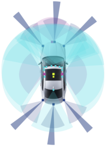
End-to-end Monitoring of Modern Cloud Applications


Introduction

During the last semester and as part of my Master’s thesis, I worked at an automotive company on the development of a vehicle connectivity platform. Within my team I was assigned the task of monitoring, which turned out to be a lot more interesting but at the same time way more complex than I expected. In this blog post, I would like to present an introduction to system health monitoring and describe the challenges that one faces when monitoring a cloud-based and highly distributed IoT platform. Following that I would like to share the monitoring concept that was the result of my investigation.

Monitoring

When developing an application, monitoring usually is not the first topic to come up to the developers or managers. During my time in university, whenever we had a fixed date to present results as part of a group’s project, me and my colleagues usually shifted our focus towards feature development rather than testing and monitoring. The need for monitoring however, becomes extremely important as soon as you have to operate a software system. Especially when maintaining distributed systems which cannot be debugged as traditional, monolithic programs the need for enhanced monitoring grows. The biggest difficulty with monitoring, is that it has to be designed specifically for the application that is needs to be monitored. There is no one-size-fits-all solution for monitoring. Within the scope of monitoring, there are a lot of different use cases to focus on. When talking about operating a software platform, our focus relies on system health monitoring.

System health monitoring

Monitoring has a different meaning depending on the domain it is being employed in. Efforts when monitoring software systems can put special interest into topics concerning security, application performance, compliance, feature usage and others. In this post I would like to focus on system health monitoring, following the goal of watching software services’ availability and being able to detect unhealthy states that can lead to service outages.

Even when reduced to health monitoring, one implementation of monitoring can differ strongly from another, depending on how different the systems, the processes, the tools and the users and stakeholders of that monitoring information are defined. The basis for monitoring is constantly changing due to the introduction of new technologies and practices. Therefore, a state of full maturity for monitoring tools can hardly ever be reached.

Monitoring Tools

Monitoring tools were created and adapted to fit for the domain of the systems that had to be monitored. Monitoring requirements are substantially different when monitoring clusters of homogeneous hardware running the same operating systems to those when managing the IT-infrastructure of a middle to large-size company with heterogeneous hardware (e.g. databases, routers, application servers, etc.).

If you are building a new software application or have been assigned the task of maintaining one, here are a few example tools that focus on different aspects of monitoring that could be interesting to try out.

  • Collectd – Push based host metric collection: Collectd is able to collect data from dynamically started and stopped instances. It works by periodically sending host metrics from preconfigured hosts to a central repository. By being a push-based system, it works also for short-lived processes. [2]
  • StatsD – Application level metric collection: StatsD was designed as a simple tool that collects traces and sends them via UDP to a central collector, where they can be forwarded to a collection and visualization tool like Graphite to be used to render graphs that are displayed in dashboards. [3]
  • The Elastic-Stack – Log management and analysis: When applications are hosted inside containers running on separate hosts, it is not only difficult to extract a containers low-level metrics, but also to extract and collect application-level metrics and logs. The standard open-source solution for this problem is the Elastic-Stack.
  • Riemann – Monitoring based on Complex Event Processing: Riemann differentiates itself from other monitoring tools in that it introduces event stream processing techniques to monitoring. Riemann works by processing events that are pushed by many distinct sources and, thanks to its push-based architecture, provides high scalability.
  • New Relic – Monitoring solution as SaaS: New Relic is one of the more recent SaaS solutions that have emerged in the past years. The feature of MaaS (Monitoring-as-a-service) is that the infrastructure and services needed to implement monitoring tools is abstracted away from operations teams. MaaS systems like New Relic can be configured to watch the infrastructure running services and receive monitoring data from the monitored objects either via data pushes directly or by installing agents that run inside hosts. Apart from collecting and processing logs, New Relic provides a browser based interface to access data and create customized dashboards as well as features like auto-detecting anomalies with the use of machine learning.
  • Zipkin – Distributed tracing: Zipkin, among other distributed tracing solutions, focuses on tracking requests on a distributed system in order to inspect the system for errors or performance bottlenecks and to enable troubleshooting in architectures where multiple components are being employed.
    Zipkin supports the OpenTracing API. OpenTracing is a project aimed to introduce a vendor-neutral tracing specification. Its objective is to standardize the tracing semantics to allow for better distributed tracing capabilities across frameworks and programming languages. Trace collectors can implement the OpenTracing API and can thereby be employed in large scale distributed systems, in which system subcomponents are written by different teams in different languages.

If your project if focused more on infrastructure components, it would be interesting to take a look at collectd. For a smaller web application, I would recommend to build in StatsD and focus on tracking relevant business KPIs from inside the relevant functions within the code. For any software project I would recommend to employ a log management system like the Elastic-Stack or an alternative. Since its an open source solution, there are no licence costs attached and it can notably reduce troubleshooting time when debugging your application, specially if your application relies on a microservice architecture. For start-ups with smaller cloud projects going to production, I would recommend trying out a Monitoring-as-a-service solution to analyze your application usage. Especially for smaller businesses going to the cloud, finding out how your customers are using your application is crucial. Discovering which functions and to what extent resources are being utilized can enable operations teams to optimize the cloud resource allocation while providing the business with important feedback about feature reception.
If you are building a complex distributed architecture involving many different components, it might make sense to evaluate more versatile tools like Riemann and take a look at OpenTracing.

Monitoring Strategy

Unarguably, the employment of the right tools or solutions to monitor a distributed system is crucial for the successful operation of it. However, effective monitoring does not only focus on tooling, but rather incorporates concepts and practices derived from the experience of system operations in regard to monitoring, and to some extent, to incident management. If your task is to monitor a software system, the best way to start is to define a monitoring strategy. When doing so, it should consider the following concepts:

  • Symptoms and causes distinction – The distinction of symptoms and causes is especially important when generating notifications for issues and defining thresholds for alerting. In the context of monitoring, symptoms are misbehavior from a user perspective. Symptoms can be slow rendering web pages or corrupt user data. Causes in contrast are the roots of symptoms. Causes for slow rendering web pages can be unhealthy network devices or high CPU load on the application servers.
  • Black-box and white-box monitoring – Black-box monitoring is about testing a system functionality and checking if the results are valid. If results are not what was expected, an alert is triggered. White-box monitoring is about getting information about a component’s state and alerting on unhealthy values. While white-box monitoring can help the operations personnel find causes, black-box monitoring is used to detect symptoms.
  • Proactive and reactive monitoring – In relation to black-box and white-box monitoring are the concepts of proactive and reactive monitoring. Whereas reactive monitoring is concerned about collecting, analyzing and alerting on data that can reflect an outage of the system, reactive monitoring emphasizes on detecting critical situations within the monitored object that can lead to a service performance degradation or complete unavailability. While the results from black-box monitoring can be useful to detect problems affecting users, white-box monitoring techniques provide more visibility into a system’s internal health state. With careful analysis of trends on internal metrics, a prediction of imminent failures can be made, which can either trigger a system recovery mechanism, an auto-scale of system resources or alert a system operator.
  • Alerting – Alerting is a crucial part of monitoring. Alerting however, does not necessarily involve paging a human being. The latter should mostly remain the exception and only be employed when services are already unavailable or failure is imminent without human action. For events that require attention, but do not involve failing systems, alerts can simply be stored as incidents in a ticketing system, to be reviewed by the operations team when no other situation requires their attention. In case of pages, they should be triggered as sparsely as possible, since constantly responding to pages can be frustrating and time consuming for operations employees. When defining thresholds to be notified on, new approaches propose to aggregate metrics and generate alerts on trends, instead of watching simple low-level metrics, e.g. watching for the rate in which available space on a database is filling up, instead of its current free space at a certain point in time. This concept relates to focusing on symptoms rather than causes when alerting.

When implementing the monitoring strategy for your project, it’s best to start with black-box monitoring, covering the areas that affect your users the most (such as being able to log in to your system). When defining alerts, focus should rely on symptoms rather than causes, since causes might or might not lead to symptoms. Also, if your are defining alerts, always focus on the right choice of recipients. Different groups of project employees might be interested on different types of alerts or different granularity. Alert the business about decreasing page views and not about cluster certificates that will expire soon.

Real-life scenario: monitoring a cloud-based vehicle connectivity platform

The connectivity platform I worked on provides infrastructure and core services to develop connectivity services for commercial vehicles. These services enable users to open the vehicles’ doors remotely via smartphone or displaying the position and current state of a vehicle on a map. The platform provided a scalable backend which handled the load of incoming vehicle signals and provided it as JSON data from APIs. It also included frontend components which fetched data from the provided APIs and displayed it in a smartphone in the custom app or in a browser as a web application. The platform was built on top of Microsoft Azure and was based on the IoT reference architecture proposed by Microsoft in the Azure documentation. It was built on a highly distributed microservice architecture that made extensive usage of Azure’s products, both SaaS and PaaS. Its core was made of an Azure Service Fabric cluster running all microservices that implemented the business logic of the connectivity services. The communication between microservices was established either synchronously via HTTP or asynchronously using Azure’s enterprise messaging component Azure Service Bus. In order to implement most use cases the platform’s components also had to communicate with various company-internal systems, as well as third party software services that implemented specific functionality, such as user management.

Monitoring challenges

In order to reach a basic level of monitoring in the platform, at least each component of the platform, which was not being fully managed by Microsoft or a third-party service provider (e.g. a SaaS- component), had to be monitored by the operations team. As stated above, special care was put in the choice of components that demanded the lowest level of administration effort of the aforementioned team. That led to an increased usage of PaaS-components instead of Virtual Machines or other infrastructure alternatives.

Even though the infrastructure of PaaS-components does not need to be managed by the cloud consumer, there are some aspects when using PaaS-components that can generate errors in runtime and must, for this reason, be constantly monitored by the operations team. Some examples are:

A queue in the Service Bus, filling up rapidly because a microservice is not keeping up with the number of incoming messages.

An Azure Data Factory Pipeline that stopped running because a wrong configuration change removed or changed a database’s credentials and the pipeline is not able to fetch new data.

The former scenario can be easily detected, since Azure provides the resource owner with many metrics regarding the high-level usage of each component. In this case, a counter of unread messages is available in the Azure Portal or via Azure Metrics. Since the counter is available in the portal, widgets displaying its data can be pinned to a dashboard and alerts can be created for a given threshold on this metric.

In the data pipeline scenario, an outage can be detected by setting alerts on the activity log, which is the only place where occurring errors within Data Factories are reported. However, an aspect adding risk to the latter scenario is that detecting that a pipeline stopped running is especially difficult when testing the system from the user’s perspective, since it is only reflected by outdated or incorrect data, instead of directly throwing an error.

In this sense, the operations team of the platform should always be notified in the case of a stopped pipeline because user complains might be misleading. Also, the advantage of using PaaS components and having the underlying infrastructure abstracted away from the user comes with the disadvantage that all available logs and metrics, from which monitoring events can be derived, are defined by the component’s provider and cannot be easily expanded, customized or complemented with own information.

The monitoring strategy

When defining the monitoring strategy for the platform from a technological point of view, the first decision was to make extensive use of the SaaS monitoring solutions already provided by Microsoft to monitor applications and infrastructure hosted inside of Azure, before introducing external proprietary solutions or deploying open-source monitoring tools to watch the platform. The tools employed were Azure Monitor, Azure Log Analytics and Azure Application Insights. Implementing white-box monitoring was simpler due to the seamless integration of tool provided by Microsoft to monitor Applications on Azure. Implementing black-box monitoring to be able to tell that the most important functions of the platform were available was way trickier. The next section explains the concept developed as part of my thesis.

End-to-end black-box monitoring

Why monitoring single components is not enough

The problem statement above only describes the challenges of monitoring each component on its own. The services offered by the platform however, are provided only as a result of the correct functioning of a specific set of these subcomponents together. In many cases, the platform’s subcomponents receive messages, process them and then forward them via a synchronous or asynchronous calls to the next subcomponents, forming complex event chains. These event chains can also include third party systems operated within the same organization or third parties, which handle specific technical areas of the connected vehicle logic. From an operations’ perspective, the most valuable information is to know whether a specific, user-facing service is running at the moment or if it is facing technical disruptions. In this case, not only knowing if a service is running in the sense of a passing an integration test is important, but rather having further insights into the system (including its complex event chains) and which part of it is failing to process the requested operation.

This observability can be partially provided by monitoring the platform’s subcomponents on their own, but not entirely. Here is one example:

In case a Service Bus queue filles up, the cause of messages missing in the frontend can be detected by alerting on a threshold on the involved Service Bus queue’s length.

However, here is an example of a case in which finding out the root cause of a service disruption might become less obvious:

A configuration change from a deployment altered the expected payload of a microservice, and incoming asynchronous messages are being ignored by that microservice for being badly formatted.

The error would only be visible by examining the logs generated by the service. If the message drop is not being actively logged by that specific microservice, there is no way for the operations team to find out on which part of the system the messages are being lost. This
observability problem is increased by the fact that PaaS components do not generate logs for every message being processed. That means the last microservice which created logs including the message’s ID is the last point of known correct functioning of the event chain.

This case might not seem probable, but most of the disruptions happening in a production environment come from unintentional changes to the configuration made by an update. Also, as the architecture becomes more and more complex and further components are added to support the main services of the chain, the task of troubleshooting the platform grows in complexity. An end-to-end black-box monitoring system, which monitors the core services of the platform, would substantially reduce effort when searching for misbehaving components since it would alert the operations team as soon as one of the core services is not available. The alert would as well include information about the exact subcomponent responsible for the outage.

What we need is Event Chain Monitoring

The core of the proposed solution is based on event correlation. In this case, an own definition of events and their aggregation was used. The core ideas are inspired by the Complex Event Processing paradigm but its full complexity would go beyond the scope of this blog post. The use of events creates an abstraction level between incoming signals and relevant information for monitoring. Sources of events can be either HTTP requests triggering a component or logs being added to the log repository of the platform or any kind of process that can be converted to an event. To map data to an event, it has to contain information that can be derived to at least the following event metadata:

  1. Event source
  2. Event timestamp
  3. Tracking ID
  4. Event type

The event source is used to map the event to the component which originally generated the event. The timestamp contains the time in UTC at which the event was generated or processed. The tracking ID is used to correlate events that belong to the same action. Using a tracking ID, all events originated by the same operation can be grouped together. The event name states the type of event that was triggered, such as data from vehicle received at gateway or message processed by microservice A.

When triggered, all events have to be routed to central repository for analysis and aggregation. From this central repository, single events can be analyzed for patterns that indicate system failures.
Defining the model for a fully functioning event chain is then simple. It is calculated with a query as the aggregation of any number of events and a syntax stating the order and time frames in which the events need to reach the central repository. The exact count of events and their order depends on the level of granularity to which the event chain is going to be monitored.
A visualization of the proposed solution is presented in the following diagram using a sample event chain:

After the event chain is modelled in the monitoring web application, the flow of events can be tracked. First, signals have to be generated. Since generating real signals would involve driving around in a real car connected to the backend, a vehicle has to be simulated, thus the first event would come from a vehicle simulator. After vehicle data events start being pushed to the platform, the different components of the system will start processing the incoming data and interacting with other subcomponents. For each subcomponent, the telemetry capabilities have to be defined. If it supports generating an event for every data signal and sending it to the central event repository or if the event hast to be generated out of the logs or other information sources that are filled by this subcomponent. Depending on the type of components and the level of administration needed, there is more or less information available. If crucial information is missing from a component, a helper or observer unit (here the “observer” Azure Functions) has to be added to the chain, to provide the missing information.

After events are matched, their results can produce other, higher-level events. These high-level events can be consumed by a monitoring dashboard, or a ticketing system. If consumed by a custom dashboard, monitoring information can then be presented by visually showing a graph of the subcomponents of the system. Depending on the patterns matched by predefined queries, different parts of the event chain, that get recognized as failing, can be highlighted in the dashboard.
In addition to displaying a graph of the event chain, the operations team can subscribe to changes to the use-cases health state. If a disruption of a core service is registered, a text message can be sent to the person on-call. Less crucial incidents can be tracked in a ticketing system for further investigation by the operations team. A further advantage of having the event chains displayed visually to the operations team is that even without deep knowledge of the platform, the operations team is able to reason about symptoms visible by users of the platform and track back many incidents that might have the same origin. That is, the operations team would get direct visibility into the state of the subcomponents of the platform and, in the case of an outage, the team gets direct information about the outage’s repercussion on the operability of the system.

Conclusion

The implementation of modern software architecture patterns like microservices combined with the use cloud services beyond IaaS facilitates a faster development of software services. Despite the reduced effort to manage infrastructure when deploying applications to the cloud, being able to monitor the resulting highly distributed systems is becoming an increasingly complex task. On top of that, customers of modern online applications expect short response times and high availability, which raises the need for accurate monitoring systems. In this post I provided a short introduction to monitoring and an overview of current monitoring tools you can test in your projects. However, I also described how a well-thought monitoring strategy is more important than tools in order to increase your system’s availability. In the second half of this post I provided a real-life example scenario and depicted the challenges related to monitoring a distributed IoT-platform. I then presented the concept that was developed in order to reach a better state of observability into the platform.

References

Some of the ideas summarised in this blog post were originally presented in the following articles or books. They are also excellent reads in case the topic of monitoring got your interest.

  • B. Beyer, C. Jones, J. Petoff, and N. R. Murphy, Site Reliability Engineering: How Google Runs Production Systems. “ O’Reilly Media, Inc.,” 2016.
  • M. Julian, “Practical Monitoring: Effective Strategies for the Real World,” 2017.
  • J. Turnbull, The art of monitoring. James Turnbull, 2014.
  • I. Malpass, “Measure Anything, Measure Everything,” 2011. link.
  • J. S. Ward and A. Barker, “Observing the clouds: a survey and taxonomy of cloud
    monitoring,” J. Cloud Comput., vol. 3, no. 1, p. 24, 2014.
  • B. H. Sigelman et al., “Dapper, a Large-Scale Distributed Systems Tracing Infrastructure,” 2010.

Reproducibility in Machine Learning

The rise of Machine Learning has led to changes across all areas of computer science. From a very abstract point of view, heuristics are replaced by black-box machine-learning algorithms providing “better results”. But how do we actually quantify better results? ML-based solutions tend to focus more on absolute performance improvements (measured by metrics) instead of factors like resilience and reproducibility. On the other hand, ML models have a significantly growing impact on humans. One can argue that the danger is negligible for applications like playing games but with direct impacts like self-driving in production, there comes a responsibility. This responsibility was strengthened not only by laws such as the EU General Data Protection Regulation (GDPR).

Nevertheless, the objective of this post is not to philosophize about the dangers and dark sides of AI. In fact, this post aims to work out common challenges in reproducibility for machine learning and shows programming differences to other areas of Computer Science. Secondly, we will see practices and workflows to create a higher grade of reproducibility in machine learning algorithms.

Background

Having a software engineering background, my first personal experience of programming in machine learning felt like going back in time. Many frameworks are evolved and highly used in practice (TensorFlow, keras, pytorch, …) but other’s are still in the early stages and evolve quickly. This fact shouldn’t be surprising regarding the short history of current ML implementations. However, the definition of frameworks differs from other areas of Computer Science. Tensorflow and others create an abstraction layer for the underlying mathematical operations and indeed simplify processes like training, optimizations and more. But for me, they are closer to a toolkit of operations than a cookbook with best-practices.

Especially scientific results are often implemented with the same toolkit but as a standalone project. For this reason, the grade of reusability of such implementations is often low. Research scientists are interested in the most recent publications but there is no baseline project which can be used for different approaches, models and datasets. It’s more about copying and pasting workflows, downloading datasets and hacking it together. However, the research in ML is now establishing programming paradigms which exist in other parts of computer science for decades. Further, I am thankful to anyone contributing to state-of-the-art implementations in the first place. Thus, we will move the scientific scope into the background from now on.

Taking a more practical approach into account, Jupyter notebooks are often used as a starting point to explore data and different approaches. They are a great tool to evaluate a proof-of-concept and to showcase initial findings. However, notebooks tend to be chaotic with increasing complexity. In certain aspects, we can compare the workflow to creating an MVP in software engineering. You can reuse the created MVP as a setup for the productive application, but you shouldn’t expect a clean and extensible architecture then.

A machine learning workflow

For a better understanding, the following figure shows a typical workflow and the components of development in Data Science:

  1. Load and preprocess data, bring it into an interpretable form for our ML model.
  2. Code a model and implement the block-box magic that empowers AI.
  3. Train, Evaluate and fine-tune the model over days, weeks or months.
ML workflow
https://cloud.google.com/ml-engine/docs/tensorflow/ml-solutions-overview

After an initial implementation and similar to software lifecycles, we have the following steps:

  1. Deploy the program (model) to our dedicated infrastructure (Cloud, local).
  2. Use the model in production.
  3. Monitor the application and its predictions.
  4. Maintain the source code, implement new features and deploy new versions.

Frameworks like TensorFlow provide tools to read data, train models and evaluate them with different metrics. Further, approaches like TensorFlow Serving address the second part of the workflow to deploy models on infrastructure for production. Nonetheless, these tools don’t explicitly address reproducibility issues in ML. For a better understanding, the following section goes one step back by pointing out these challenges.

Challenges in ML reproducibility

In contrast to other fields of computer science, the results are non-deterministic. In other words, the same source code produces different results for the same dataset. Reasons mostly lie in implementation details such as random initializations of parameters or randomly shuffled datasets.

However, the baseline for collaboration in software engineering is a project environment where changes can be reproduced. There is not enough time in this blog post to discuss concepts like Versioning and Continous Integration, but in general, they lead to projects that are less error-agnostic due to automatic testing and deploying. Furthermore, contributors are able to comprehend changes and reproduce it on their environment (if guidelines and rules are followed).

Having the non-determinism in mind, the  objective for ML is a process in which results can be produced having the exact same results. The following aspects address this issue:

  1. Versioning of models: Models should be versioned and any changes be transparent.
  2. “Results without context are meaningless.“ (https://www.pachyderm.io/dsbor.html). For reproducibility, the collection of metadata is essential. Running a model on a dataset and versioning it does not answer questions such as: Where did the data come from? How can we rerun the model with an updated dataset?
  3. A reproducibility flag should enable a mode in which features causing non-deterministic results such as random initialization are disabled.

Coming back to Jupyter notebooks as a baseline for ML projects, they are a nightmare from a versioning and reproducibility perspective. First, notebook cells can run in different orders which makes the results hard to understand. Secondly, the actual source of notebooks is illegible which basically means that one can’t understand changes between versions regarding the source code. So as software developer, just imagine checking out a version and searching for changes in the application because source differences are meaningless.

So, how in practice?

We have gained an intuition for challenges in ML development and learned that versioning and collecting metadata is crucial for reproducibility. We are now answering the question of how to address these issues with in practice.

Data versioning tools

Data version control (DVC) or datmo are open source production tools for model management. In other words, they are versioning tools similar to git but address additional data scientist needs. One fundamental need is the integration of large files from different data sources. Git is not made to handle large files and the source for machine learning data is often on a different source (Public Cloud, Customer’s infrastructure).

Thus, the Git Large File Storage (LFS) replaces large files such as data input files with text pointers inside Git and stores the data on a remote server. Going one step further, we don’t want the data as part of the tool but the entire workflow. For a better understanding, the following figure illustrates a very basic scenario for DVC.

https://dvc.org/doc/use-cases/data-and-model-files-versioning

We publish and check out the code using a remote hub (Gitlab, Github, …) just as usual. On top of this, we use DVC to publish and retrieve data versions using a different hub. This separation of code and data makes it possible to test different program versions on various data versions. This is particularly useful to reproduce a model’s performance over time in production (after collecting new data).

On top of this, the tools address the following features (not exclusively):

  • Language- and Framework-agnostic: Implement projects in different languages (Python, R, Julia, ..) using different frameworks (TensorFlow, PyTorch, …)
  • Infrastructure-agnostic: Deploy models to different environments and infrastructures (Google Cloud, AWS, local infrastructure)

However, the infrastructure-agnostic feature comes with a drawback. DVC or datmo lack pipeline execution features for build pipelines, monitoring or error handling. The philosophy of these tools is to be very generic without running servers. They are slim command line tools without user interfaces.

Pachyderm

In order to come closer to continuous integration, we need deployment pipelines and modular infrastructure. The goal is an automated processes of releasing new versions, testing it on a staging environments and deploying it to customers. The borders between infrastructure and programming are blurring and the same should apply to machine learning. The two keywords that pop up in every (modern) infrastructure are containers (docker) and Kubernetes. Say hi to Pachyderm.

Pachyderm runs on top of Kubernetes which makes it deployable to any service that supports Kubernetes (Google Cloud Platform, AWS, Azure, Local infrastructure). Further, it integrates git-like features to version code as well as data and it shares many of its names (repository, pipeline, …). With Pachyderm, we configure continuous integration pipelines with container images.

Image result for pachyderm data science
https://www.slideshare.net/joshlk100/reproducible-data-science-review-of-pachyderm-data-version-control-and-git-lfs-tools

The above figure shows a baseline workflow in Pachyderm. Assuming that we already created a repository and coded our model, we put a file to our dedicated data storage. We then create pipelines whose configurations are written as JSON-files and can look as follows:

{
  "pipeline": {
    "name": "word-count"
  },
  "transform": {
    "image": "docker-image",
    "cmd": ["/bin", "/pfs/data", "/pfs/out"]
  },
  "input": {
      "pfs": {
        "repo": "data",
        "glob": "/*"
      }
  }
}

By executing the above configuration with the Pachyderm command line interface pachctl create-pipeline -f above_pipeline.json, we run the commands in cmd within the container created from an image defined in image. Further, we use remote storages like S3 or store it on the Pachyderm File System (pfs). PFS is a distributed filesystem which is, until a certain level, comparable to the Hadoop file system (HDFS) where MapReduce-Jobs are replaced by Pachyderm pipelines (see 8).

After creating the pipeline above, Pachyderm will launch worker pods on Kubernetes. These worker pods will remain up and running, such that they are ready to process any data committed to their input repositories.

KubeFlow: Distributed large-scale deployment

As described beforehand, Pachyderm let us create scalable and manageable ML pipelines on Kubernetes. Although Pachyderm can be parallelized in a map/reduce-style way, the pipelines mostly rely on single nodes and non-distributed training (multiple GPUs, but not multiple nodes). Having a different approach in mind, KubeFlow mainly focuses on standards to deploy and manage distributed ML on Kubernetes. It integrates tools like Distributed TensorFlow or TensorFlow Serving and further JupyterHub which improves the process of developing in teams on shared notebooks.

However, KubeFlow (as of now) lacks tools that orchestrate Data Science workflows as seen earlier (Data Preprocessing, Modelling, Training, Deployment, Monitoring, …). It leaves these responsibilities up to the developer. Since this blog post mainly focuses on reproducibility in Machine Learning, KubeFlow does not answer these questions satisfactory. Consequently, further concepts are out-of-scope for this post while not being less exciting for productive and large-scale ML engineering.

Nevertheless, reproducibility and productivity should go hand in hand. For this reason, KubeFlow and Pachyderm can be jointly used in practice. In such a scenario, Pachyderm would provide the reproducibility through pipelines and KubeFlow would bring with the ease of deployment and distributed framework integrations (see 67 for more details).

So what should I use?

After an introduction to tools such as DVC and Pachyderm, one last question remains: Which is the best tool in production? And as always the answer is – it depends. DVC can improve productivity in smaller teams to organize and version projects and link the source code to the data. However, for organizations willing to introduce a workflow, richly-featured tools such as Pachyderm are the way to go. Taking one step further, KubeFlow paves the way for large-scale and distributed applications.

From a different point of view, the discussion behind it could be seen as a discussion about Kubernetes itself. This is fairly more wide-reaching and asks fundamental questions such as: Can we pay someone to set up and maintain the Kubernetes Cluster? Are our applications and workflows complex enough (multiple nodes, not multiple GPUs) to justify the overhead of Kubernetes? Unfortunately, we can’t answer these questions in this blog post.

Wrapping it up

In Machine Learning, programs can have the same meaning and even speak the same language but output different results because context matters and implementations are full of (intended) randomness. Further, development in ML is very sensitive to changes and even small differences can have high impacts on the result. For reproducibility, we have to record the full story and keep track of all changes.

Frameworks such as DVC or Pachyderm help to keep track of not only the code but also the data. Furthermore, they use pipelines to reproduce results and simplify collaborative projects. This increases the reproducibility and corresponds to the responsibility in ML. On top of this, the tools are a first step towards the fulfillment of laws like the GDPR because results can at least be reproduced. However, these solutions are to some extent immature and evolve quickly (however, just like everything else in ML). It is still a long way to go to obtain practices in ML which are comparable to standards in software engineering.

Related Sources and further reading

  1. Collaboration Issues in Data Science (accessed: 25.02.19): https://github.com/iterative/dvc.org/blob/master/static/docs/philosophy/collaboration-issues.md
  2. Hold Your Machine Learning and AI Models Accountable (accessed 25.02.19): https://medium.com/pachyderm-data/hold-your-machine-learning-and-ai-models-accountable-de887177174c
  3. How to Manage Machine Learning Models (accessed: 25.02.19): https://www.inovex.de/blog/how-to-manage-machine-learning-models/
  4. Introducing Kubeflow – A Composable, Portable, Scalable ML Stack Built for Kubernetes (accessed: 26.02.19): https://kubernetes.io/blog/2017/12/introducing-kubeflow-composable/
  5. Machine-Learning im Kubernetes-Cluster (German, accessed: 25.02.19): https://www.heise.de/developer/artikel/Machine-Learning-im-Kubernetes-Cluster-4226233.html
  6. Machine Learning Workflow (accessed: 26.02.18): https://cloud.google.com/ml-engine/docs/tensorflow/ml-solutions-overview
  7. Pachyderm and Kubeflow integration (accessed: 26.02.18): https://github.com/kubeflow/kubeflow/issues/151
  8. Pachyderm File System (PFS, accessed: 26.02.18): https://docs.pachyderm.io/en/v1.3.7/pachyderm_file_system.html
  9. Provenance: the Missing Feature for Rigorous Data Science. Now in Pachyderm 1.1 (accessed 25.02.19): https://medium.com/pachyderm-data/provenance-the-missing-feature-for-good-data-science-now-in-pachyderm-1-1-2bd9d376a7eb
  10. Reproducibility in ML: Why It Matters and How to Achieve It (accessed: 25.02.19): https://determined.ai/blog/reproducibility-in-ml/
  11. Reproducible data science: review of Pachyderm, Data Version Control and GIT LFS tools (slides, accessed: 25.02.19): https://www.slideshare.net/joshlk100/reproducible-data-science-review-of-pachyderm-data-version-control-and-git-lfs-tools
  12. The Data Science – Bill of Rights (accessed: 25.02.19): https://www.pachyderm.io/dsbor.html

Experiences from breaking down a monolith (1)

Written by Verena Barth, Marcel Heisler, Florian Rupp, & Tim Tenckhoff

The idea

The search for a useful, simple application idea that could be realized within a semester project proved to be difficult. Our project was meant to be the base for several lectures and its development should familiarize us with new technologies and topics. Someday a team member was standing at a train stop, waiting for the delayed subway to finally arrive and came up with the idea that it would be interesting to see statistics about the average/total delay of the Deutsche Bahn!

This is how the idea was born: We wanted to develop a device-independent web application to visualize both, the average and the accumulated delay, as well as current departures of the public transportation at some stops. Our application called Bahnalyse receives its data via the VVS API. To calculate the statistics, the departure times of the railways are crawled in a regular time interval and stored in a database. To search for station names as well as to display the current delays, the VVS API is called directly.

During the lecture “Web Application Architecture” we thought about a first simple application architecture, patterns and technologies we wanted to use. This was significantly influenced by the lecture “System Engineering and Management”, in the context of which this blog post is written.

General aims, technologies

Our aims for this lecture were initially to get in touch with CI/CD, Docker and the deployment to the Cloud – topics that are currently on everyone’s lips and with which we haven’t had much to do yet. Furthermore we wanted to improve the architectural concept of our quite simple application, e.g. by splitting it up, decouple the components from each other and experiment with different types of databases.

For the development we chose Angular and made use of some other useful npm packages including ng2-charts (offering Angular directives for Charts.js which provide HTML5 based, animated JavaScript charts) and Angular Material, which offers modern UI components following Google’s Material Design spec. The Java backend was developed with Spring Boot making it easy to create stand-alone applications without much XML configuration. Initially we wanted to realize a relational MySQL database in combination with Hibernate. But let’s see where the system engineering process took us to. 😉

Which cloud provider fits best?

Since deploying to the cloud was one of our initial goals, we started to look for the “best” cloud provider early. We compared the most common ones (in Europe and US) AWS (Amazon Web Services), IBM Cloud, GCP (Google Cloud Platform) and Microsoft Azure in four Categories.

The first category is Enterprise Adoption because it makes sense to learn and try out the cloud provider we will use most likely later on at work. We found a study from Right Scale about this topic where AWS is clearly the leader. 68% of the 997 participating companies from different industries were running applications on AWS in 2018. The second place made Azure with 58% but this might be misleading because it includes Office 365 customers which is not interesting for us.

Category two is documentation. We found a blog post from a fellow student from July 2018 that says “documentation is key”. He tried out AWS, GCP and IBM and again AWS won with a “Still bad documentation but best of all“. Of course this is only his point of view but at least he had tried them out before judging. So for us his opinion gives us at least a good clue.

The third category is the community. Therefore we compared the amount of questions asked on Stack Overflow of all time. If there are already a lot of questions asked the possibility grows, that means the questions we might have would have possibly been answered already. Again the winner is AWS with 65,427 questions. We did not consider the percentage of unanswered questions, because it is not differing very much between the cloud providers. We looked up those numbers in October 2018.

The last but most important category are costs. Being students just trying out some technologies we did not want to spend any money. So we only compared free tiers and student accounts we did not check out what it would cost to run our application for a longer time.

We started by trying out the AWS Student Account. Given only the Starter Account by the Stuttgart Media University (HdM) we don’t have access to any IAM-Tools. Also it is not possible to create access keys for our user. This and the federate login of the student account itself made logging in from a CI-Pipeline impossible. Thus the AWS student account became useless for us. The AWS free tier would probably provide the features we need for free up to 12 month and up to a limited amount of resources. But it requires a credit card for registration that will be charged if any of the free tier limitations are exceeded. There is no possibility to set any limits for the payments so it’s not possible to say “shut down all my instances before I would have to pay for them”.

For the GCP student accounts we are not enabled because our university would have to apply for it first. The free tier also requires a credit card. But at least it will only be charged after confirmation when the free tier is used up.

Still we did not want to provide a credit card at all. Luckily IBM Cloud provided exactly what we are looking for. A six-month free student account with no need to provide a credit card and only few limitations on the available features. To activate it you need to get a promo code and supply it in your free account to upgrade to a student account.

The table below shows an overview of the categories explained above. The last row contains additional considerations. So we were told that containers are running in actual Kubernetes Clusters on GCP whereas AWS uses VMs. Also we read that GCP provides the “best AI” services, but this does not matter for our use case.

Finally we can conclude that we would use IBM Cloud because of the free student trial. But actually we did not deploy to any cloud so far. While working on the project we found other interesting topics we concentrated on and deployed the old-fashioned way to a server we got from the HdM also for free.

AWSIBMGCPAzure
Enterprise adoption 68%15%19%58%
Documentation “bad but best“bad”
„little bit better“
Community 65.427 5.256 10.352 62.638
Free? Student account: useless
Free tier: credit card required, no limits possible
Student account: few limitations, six month free Student account: HdM not applied
Free tier: credit card required confirm paid account, few limits possible
Miscellaneous VMs Kubernetes,
best AI Services
Mainly Office 356 customers

Experiences from breaking down a monolith (2)

Written by Verena Barth, Marcel Heisler, Florian Rupp, & Tim Tenckhoff

Architecture

Besides earlier technological considerations, we primarily wanted to change the architecture of the initial project. The first approach was in spite of the applied software patterns and architectural concepts of the Web Application Architecture lecture constructed as a monolith. That means in fact, that the whole logic was written in one software layer, providing worst conditions for scalability or expandability. For this reason, we decided to decouple the logical components of our software.

This distribution resulted in a separation of frontend and web backend, and the relocation of smaller logical parts of the software into microservices: An implemented database service contains logic to process all upcoming database requests to store or to access data. The Crawler service is designed to control the periodic queries to the VVS API to request the delay information. Through the implementation of these microservices, we broke down the functionality of these software components to the smallest possible dimension in accordance with the principle of software oriented architecture (SOA). Thus, we consequently increased the possibility to scale, maintain or exchange subcomponents of our code. Additionally, we reached a separation of components that could possibly slow down each other (e.g. if subcomponents require database access at the same time). The final architecture is shown in figure 1.

Figure 1: Final application architecture

Message Broker

So we decided to build a distributed system based on service oriented architecture (SOA). In earlier times building monolithic software, nobody wasted any thought on how to let parts of the software talk to each other. This was easy – the source code to be called was just directly available. Compared to a distributed system, things changed now. As its name already tells you, services in a distributed system are at least separated by software and often also by hardware infrastructure. It’s obvious that any communication between them now must go over the wire. To approach this problem we came along with the technology of message brokers. This piece of third party software can be imagined as a post office. All it does, is accepting messages and then routing them according to the information on the envelope to interested customers. To get experienced with the use of message brokers, we decided to use the RabbitMQ implementation. Some advantages coming up with that choice are the out of the box use, a very good documentation and interface libraries with great tutorials for most programing languages. Other message brokers you might have heard of may be Apache Kafka or ActiveMQ.

For keeping received messages encapsulated from delivery, RabbitMQ uses the pattern of exchanges. By doing so, each message is sent to a specific exchange configured on the broker with a routing key on the envelope. Now the exchange maps the message to a queue looking at the routing key. Due to this, a message could be sent to multiple queues by only sending one message for example. Of course you have to configure things properly ;-). For this reason, RabbitMQ provides multiple different types of exchanges, for example the fanout exchange. This does exactly what mentioned before – sending a broadcast. If you prefer a one-to-one communication I’d recommend you the direct exchange.

As larger your system drives, as much more complex gets the communication architecture. Good thing was, we only had three services which need a traffic connection – the web backend service, the crawler service and a database service (see also below diagram).

Figure 2: Message Broker communication

There exist two message exchange ways: The crawler must save data into the database and the web backend must be able to query this data from the database. Because of a database query is formerly triggered by an user interaction, this must be separated to avoid unnecessary traffic which may slow down the communication. So each of them gets its own exchange configuration on the exchange. Then, to save the data the crawler has fetched, it sends it to the crawler exchange with the routing key crawler-data. By its configuration the message broker knows, it must be routed to the crawler-data-queue, to which the database service listens to. Here we are using an exchange of the type fanout. This brings the advantage to be able to save the data likewise in multiple databases.

The main difference of the communication between the web backend and the database is now, that the web backend makes a query. This means it also expects an answer with data, compared to the crawler which only sends it. Thus the pattern of an remote procedure call (RPC) is known to solve this issue. Exactly one of this is sent to the dedicated database exchange, when the web backend sends a query. Things happen the same way like explained before, but now the web backend is waiting synchronously for the answer of the database.

In our example, things were still clear and easy to manage. But thinking of a system running ten times as many services with multiple instances of each, you fastly lose sight. At this point you need to think about the maximum utilisation of your system. This is where the queuing theory focuses on. By setting the service disciplines and some parameters, you are able to calculate the produced traffic inside your system.

Time Series Database

The general specifications of our project, which should allow the distributed software to store data periodically and to provide these collected data according to time based queries, led to considerations about the most suitable database system for our use case. Our initial observations resulted in the fact that the required data are on the one hand based on an information about a specific date, containing a train station and the related list of trains and their delays, and on the other hand needed to be accessible by queries that use a time range (e.g. the last week) as search parameter. As time was the key indicator in both the above cases, we began to reflect if the generally used concept of a relational database as SQL would sufficiently fit our needs. Regarding this, we quickly discovered the concept of time series databases. As the name indicates, this concept identifies points in a given data series by the factor ‘time’. Thereby it can be compared to SQL database tables where the primary key is pre-set by the system and is always the time.

Across different suppliers of time series databases we found the InfluxDB, which promises to be able to store a large volume of time-series data and to perform real-time analysis and requests on those data. Apparently, this was exactly what we needed to store and access the required information. Additionally we found a well documented tutorial, which facilitated the integration of the InfluxDB in our Spring Boot project.

The database itself could be installed and configured via the command line for local development. On our production server, we set up a docker container with a pre-configured environment, where the InfluxDB could run. A terminal interface (accessed by entering ‘influx’) allowed the manual maintenance of existing tables and their content. The InfluxDB provides a request syntax which is similar to the already known SQL query language. Therefore we didn’t need to adapt the existing data structure in our Spring Boot project to switch between SQL and InfluxDB during the development process.

One difficulty to overcome consisted of the storage of multiple trains and connections of the same time. As our service crawls data about all trains that are expected to arrive at a specific station within the next minutes, the output to store is a list of data where every object in the list correlates with the timestamp of crawling. Thus, every entry of this list theoretically had the same timestamp – and can in return impossibly be saved in a time series database, where the unique primary key is the time. To solve this, we manually added 100 milliseconds to every further entry of the timestamp and called this list of trains and their related delay a “Stop Event”. As a result, our database could possibly contain duplicate entries of trains that are delayed over a longer period of multiple timestamps. To filter out these duplicates, we needed to implement the functionality to iterate over all entries of a query result, ensuring that only the last and valid delay of a train influences the statistics in our web view.

Experiences from breaking down a monolith (3)

Written by Verena Barth, Marcel Heisler, Florian Rupp, & Tim Tenckhoff

DevOps

Code Sharing

Building multiple services hold in separated code repositories, we headed the problem of code duplication. Multiple times a piece of code is used twice, for example data models. As the services grow larger, just copying is no option. This makes it really hard to maintain the code in a consistent and transparent way, not to mention the overhead of time required to do so. In the context of this project, this issue was solved by creating an own code library. Yes, a library with an own repository which not directly builds an executable service. But isn’t it much work to always load and update it in all the services?  Yes it is – as long as you are not familiar with scripting. Therefore the build management tool gradle is a big win. It gives you the opportunity to write your own task to be executed, such like the packaging of a java code library as maven package and the upload to a package cloud afterwards. Good thing there is the free package host provider packagecloud.io around, which allows a storage size of 150MB for free. When the library was hosted online, this dependency could easily loaded automatically by the gradle dependency management.

By the use of this approach, the code development process could focus on what it really needs to – the development and not code copying! Also the team did more think about how to design the code to be more flexible, to be able to reuse it in another service. Of course it was an overhead of additional work, but the advantages outweigh. If the library is to be updated, this could achieved by an increment of its version number. Therefore all services can change only the version number and get the new software automatically updated.

CI/CD

To bring development and operations closer together we set up a CI/CD-Pipeline. Because we wanted to have a quick solution to support the development as fast as possible by enabling automated builds, tests and deployments, we had to choose a tool very early. We came up with the alternatives GitLab hosted by our University or setting up Jenkins ourselves. We quickly created the following table of pros and cons and decided to use HdM’s GitLab mainly because it is already set up and contains our code.

Our first pipeline was created ‘quick and dirty’, and it’s main purpose was just to build the projects with Gradle (in case of a Java project), to run it’s tests and to deploy it to our server. In order to improve the pipeline’s performance we wanted to cache the Gradle dependencies which turned out to be not that easy. Building the cache as the official GitLab Docs described it did not work, neither the workaround to set the GRADLE_USER_HOME variable to the directory of our project (which was mentioned very often, e.g. here and here). The cache seemed to be created but was deleted again before the next stage began. We ended up pushig the Gradle Wrapper in our repository as well and using it to build and test our application. Actually it is recommended anyway to execute a build with the Wrapper to ensure a reliable, controlled and standardized execution of the build. To make use of the Wrapper you need to make it executable (see “before_script” command in the code below). Then you’re able to build your project, but with other commands, like “./gradlew assemble” instead of “gradle build”.

image: openjdk:11-jdk-slim-sid

stages:
 - build
 # [..]

before_script:
 - chmod +x gradlew
 - apt-get update -qy

build:
 stage: build
 script:
    - ./gradlew -g /cache/.gradle clean assemble

# [..]

In the end we improved the time needed from almost four to about two and a half minutes.

Having this initial version in use we spent some more time on improving our pipeline. In doing so we found some more pros and cons of the different tools we compared before and a third option to think about.

The main drawbacks we found for our current solution were, that HdM does not allow docker-in-docker (dind) due to security reasons and GitLab container registry is disabled to save storage. In return we read that the docker integration is very powerful in GitLab. The added option GitLab.com could solve both the problems we had with HdM’s GitLab. But we came up with it too late in the project because we were already at solving the issues and didn’t want to migrate all our repositories. Also company-made constraints might always occur and we learned from solving them.

Our GitLab Runner

To solve our dind problem we needed a different GitLab Runner because the shared runners provided by HdM don’t allow docker-in-docker for security reasons. Trying to use it anyway makes the pipeline fail with logs containing something like this:

docker:dind ...
Waiting for services to be up and running...
*** WARNING: Service runner-57fea070-project-1829-concurrent-0-docker-0 probably didn't start properly.
Health check error:
service "runner-57fea070-project-1829-concurrent-0-docker-0-wait-for-service" timeout
Health check container logs:
Service container logs:
2018-11-29T12:38:05.473753192Z mount: permission denied (are you root?)
2018-11-29T12:38:05.474003218Z Could not mount /sys/kernel/security.
2018-11-29T12:38:05.474017136Z AppArmor detection and --privileged mode might break.
2018-11-29T12:38:05.475690384Z mount: permission denied (are you root?) 
*********

To use our own runner there are some possibilities:

  1. Install a runner on a server
  2. Install runners locally
  3. Integrate a Kubernetes cluster and install a runner there

Since we already have a server the first option is the easiest and makes the most sense. There are tutorials you can follow straight forward. First install the runner and then register the runner for each GitLab repository you want to allow to use this runner. The URL and token you need to specify for registration can be found in GitLab under Settings -> CI/CD -> Runners -> Set up a specific Runner manually.  It is also help provided to choose the executor, which needs to be specified on registration.

We chose Docker as executer because it provides all we need and is easy to configure. Now the runner can be started with “gitlab-runner start”. To be able to use docker-in-docker some more configuration is necessary but all changes to the config file “/etc/gitlab-runner/config.toml“ should automatically be detected and applied by the runner. The file should be edited or modified using the “gitlab-runner register” command as described here. For dind the privileged = true is important that’s why it already occurred in the logs above. Finally Docker needs to be installed on the same machine as the runner. The installation is described here. We chose to install using the repository. If you don’t know which command to choose in step 4 of “Set up the repository” you can get the information with “uname -a”. We also had to replace the “$(lsb_release -cs)” with “stretch” as mentioned in the Note. To figure out the parent Debian distribution we used “lsb_release -a“.

Pipeline Setup

Now that we solved our docker-in-docker problem we can set up a CI pipeline that first builds our project using a suitable image and then builds an image as defined in a corresponding Dockerfile.

Each service has its own Dockerfile depending on it’s needs.For the Database service image for example we need to define many environment variables to establish the connection between the database and message broker. You can see it’s Dockerfile below.

FROM openjdk:8-jdk-slim

RUN mkdir /app/
COPY build/libs/bahnalyse-database-service-1.0-SNAPSHOT.jar /app
WORKDIR /app

ENV RABBIT_HOST 172.17.0.2
ENV RABBIT_PORT 5672

ENV INFLUXDB_HOST 172.17.0.5
ENV INFLUXDB_PORT 8086

CMD java -jar bahnalyse-database-service-1.0-SNAPSHOT.jar

The frontend Dockerfile is splitted in two stages: The first stages builds the Angular app in an image which inherits from a node image version 8.11.2 based on the alpine distribution. For serving the application we use the nginx alpine image and move the dist-output of our first node image to the NGINX public folder. We have to copy our nginx configuration file, in which we define e.g. the index file and the port to listen to, into the new image as well. This is how the final frontend Dockerfile looks like:

# Stage 1 - compile Angular app

FROM node:8.11.2-alpine as node

WORKDIR /usr/src/app
COPY package*.json ./
RUN npm install
COPY . .
RUN npm run build

# Stage 2 -  For serving the application using a web-server

FROM nginx:1.13.12-alpine

COPY --from=node /usr/src/app/dist /usr/share/nginx/html
COPY ./nginx.conf /etc/nginx/conf.d/default.conf

Now let’s look at our gitlab-ci.yml file shown below:

image: docker:stable
 
variables:
  DOCKER_HOST: tcp://docker:2375/
  DOCKER_DRIVER: overlay2
 
services:
  - docker:dind
 
stages:
  - build
  - test
  - package
  - deploy
 
gradle-build:
  image: gradle:4.10.2-jdk8
  stage: build
  script: "gradle build -x test"
  artifacts:
    paths:
      - build/libs/*.jar
 
unit-test:
  image: gradle:4.10.2-jdk8
  stage: test
  script:
    - gradle test
 
docker-build:
  only:
  - master
  stage: package
  script:
  - docker build -t $CI_REGISTRY_IMAGE:latest -t $CI_REGISTRY_IMAGE:$CI_COMMIT_SHA .
  - docker login -u token -p $IBM_REGISTRY_TOKEN $CI_REGISTRY 
  - docker push $CI_REGISTRY_IMAGE:latest
  - docker push $CI_REGISTRY_IMAGE:$CI_COMMIT_SHA
 
server-deploy:
  only:
  - master
  image: kroniak/ssh-client
  stage: deploy    
  script:    
  - echo "$CI_SSH" | tr -d '\r' > pkey
  - chmod 400 pkey    
  - ssh -o stricthostkeychecking=no -i pkey root@bahnalyse.mi.hdm-stuttgart.de "docker login -u token -p $IBM_REGISTRY_TOKEN $CI_REGISTRY && docker-compose pull bahnalysebackend && docker-compose up --no-deps -d bahnalysebackend"

Compared to our first version we now make use of suitable Docker images. This makes the jobs faster and the file clearer. Most of the first parts are taken from this pretty good tutorial, so we’ll keep the explanations short here. At first we specify docker:stable as default image for this pipeline. This overrides the one defined in the runner configuration and can be overridden in every job again. Using the “services” keyword we also add docker-in-docker to this image. The variable DOCKER_HOST is required to make use of dind because it tells docker to talk with the daemon started inside of the service instead of the default “/var/run/docker.sock” socket. Using an overlay storage driver improves the performance. Next we define our stages “build”, “test”, “package” and “deploy” and then the jobs to run in each stage.

The gradle-build job now uses the gradle image with the version matching our requirements. This includes all the dependencies we need to build our jar file with “gradle build”. We use the -x test option here to exclude the tests because we want to run them in a separate stage. This gives a better overview in the GitLab UI because you see what went wrong faster. Using “artifacts” we can store the built jar file to the specified path. There it gets available for other jobs as well as downloadable from the GitLab UI.

In the test stage we simply run our unit tests using “gradle test”. This needs to compile again because we excluded the tests from the jar in our build task.

In the package stage we create a Docker image including our jar file. Using the “only” keyword we specify that this should only happen in the master branch. The first line of the “script” block uses a backend Dockerfile mentioned above in the root directory of the project (specified by the dot at the end of the line) to create the image.

For the following steps to work we need to solve our second problem: the absence of the GitLab Container Registry in HdM’s GitLab. A registry is a storage and content delivery system, holding named Docker images, available in different tagged versions. A common use case in CI/CD is to build the new image in the pipeline, tag it with something unique like a timestamp and as “latest”, push it to a registry and then pull it from there for deployment. There are alternatives to the registry integrated in GitLab we will discuss later. First let’s finish the explanations of the yaml file. We followed the just described use case of the registry. As something unique we chose the commit hash because the images get saved with a timestamp in the registry anyway. It is accessible using the predefined environment variable $CI_COMMIT_SHA. We also defined environment variables for the login credentials to the registry so that they don’t appear in any files or logs. Using environment variables like the name of the image can also help to make the registry easier exchangeable because this file could stay the same and only the variables would need to change. They can be defined in the GitLab UI under Settings -> CI/CD -> Environment variables.

In the deploy stage we used a public image from docker hub that has ssh installed so that we don’t have to always install it in the pipeline what costs time. A more secure solution would be to create such an image ourselves. We login to our server using a ssh key saved in the CI_SSH environment variable. Then run the commands on the server to login to our registry, pull the latest image and start it. To pull and start we use docker-compose. Docker Compose is a tool for defining and running multi-container Docker applications. It is mainly used for local development and single host deployments. It uses a file by default called docker-compose.yml. In this file multiple services can be defined with the Dockerfiles to build them or with the name including registry to get them from as well portmappings and environment variables for each service and dependencies between them. We use the –no-deps option to restart only the service where the image has changed and -d to detach it into the background otherwise the pipeline never stops.

Choosing a Registry

Since we cannot use the registry integrated into GitLab we considered the following alternatives:

  1. Set up our own registry
  2. Use docker hub
  3. Use IBM Cloud Registry (or other cloud provider)

The first approach is described here. Especially making the registry accessible from outside e.g. from our pipeline make this approach much more complicated than the other solutions. So we discarded this one.

Instead we started out using the second approach, docker hub. To login to it the $CI_REGISTRY variable used in the gitlab-ci.yml file should contain “index.docker.io” or it can just be omitted because it is the default for the docker login command. Besides the ease of use the unlimited storage is its biggest benefit. But it has also some drawbacks: You get only one private repository for free. To use this repository for different images makes it necessary to distinguish them using tags what is not really their purpose. Also login is only possible with username and password. So using it from a CI pipeline forces a team member to write its private credentials into GitLab’s environment variables where every other maintainer of this project can read them.

For these reasons we switched to the IBM Cloud Registry. There it is possible to create a user with its own credentials only for the pipeline using the IBM Cloud IAM-Tools or just creating a token to use for the docker login. To switch the registry only the GitLab environment variable $CI_REGISTRY needs to be adjusted to “registry.eu-de.bluemix.net” and the login needs to be updated, too (we changed from a username and password approach to the token one shown in the file above). Also the amount of private repositories is not limited and you get another helpful tool on top: Vulnerability-Checks for all the images. Unfortunately the amount of free storage is limited. Since our images are too big we got access to HdM’s paid account. So to minimize costs we had to ensure that there are not too many images stored in this registry. Since logging in to IBM Cloud’s UI and removing old images manually is very inefficient we added a clean-up job to our pipeline.

The possibilities to such a clean up job work are quite limited. There is no simple docker command for this, like docker login, push or pull. Probably the most docker-native way is would be using the docker REST API as described here. But this is only accessible for private cloud customers at IBM. The other approach described in the mentioned blogpost is deleting from the filesystem what is even less accessible in a cloud registry. So we have to use an IBM Cloud specific solution. Some fellow students of us had the same problem and solved it using the IBM Cloud CLI as described in their blogpost. We were looking for a solution without the CLI-tools for IBM Cloud and found a REST API that could do the job which is documented here. But for authorization you need a valid bearer token for which to receive in a script you need to use the CLI-tools. We chose to use this API anyway and ended up with the following additional job in our gitlab-ci.yml file:

registry-cleanup:
  stage: deploy
  script:
  - apk update
  - apk add curl
  - curl -fsSL https://clis.ng.bluemix.net/install/linux | sh
  - ibmcloud plugin install container-registry
  - apk add jq
  - ibmcloud login --apikey $IBM_API_KEY -r eu-de
  - ibmcloud iam oauth-tokens | sed -e 's/^IAM token:\s*//g' > bearertoken.txt
  - cat bearertoken.txt
  - >-
      curl
      -H "Account: 7e8029ad935180cfdce6e1e8b6ff6910"
      -H "Authorization: $(cat bearertoken.txt)"
      https://registry.eu-de.bluemix.net/api/v1/images
      |
      jq --raw-output
      'map(select(.RepoTags[0] | startswith("registry.eu-de.bluemix.net/bahnalyse/testrepo")))
      | if length > 1 then sort_by(.Created)[0].RepoTags[0] else "" end' > image.txt
  - >-
       if [ -s image.txt ] ;
       then 
       curl -X DELETE
       -H "Account: 7e8029ad935180cfdce6e1e8b6ff6910"
       -H "Authorization: $(cat bearertoken.txt)"
       https://registry.eu-de.bluemix.net/api/v1/images/$(cat image.txt) ;
       else
       echo "nothing to delete" ;
       fi

We run it at deploy stage so it could run in parallel to the actual deploy job if we had more than one runner.

First we install the required tools curl, IBM Cloud CLI and jq. This should be done by creating and using an appropriate image later. Then we login using the CLI-tools and get a bearer token. From the answer we need to cut off the beginning because it is (sometimes) prefixed with “IAM token: “ and then write it into a file. Curl is used to call the REST API with the headers for authorization to set and receive all the images available in our registry. We pipe the output to jq which is a command line tool to parse JSON. We select all the images with the same name as the one we just created. If there are already more than two we sort them by the created timestamp, grab the oldest one and write its name, including the tag, to file. If there are only two or less of these images we create an empty file. The –raw-output option of jq omits the quotes that would be around a JSON output. Finally we check if the file contains an image and delete it via API call if there is one. Somehow the else block, telling that there is nothing to delete, doesn’t really work yet. It is probably something wrong with the spaces, quotes or semicolon, but debugging a shell script defined in a yaml file is horrible so we’ll just live with our less talking pipeline. The yaml format also makes the >- at the beginning of a command necessary, otherwise the yaml is invalid. In our case an error like “(<unknwon>): mapping values are not allowed in this context at line … column …” occurred.

Conclusion

Our aims for the implementation of the application Bahnalyse was to play around with modern technologies and practices. While learning a lot about architectural patterns (like SOA and microservices), cloud providers, containerization and continuous integration, we successfully improved the application’s architecture.

We found out that the pure implementation of architectural principles is hardly possible and rarely makes sense. Although we initially wanted to split our monolith up into several microservices we ended up creating a SOA which makes use of both, a microservice and services which are composed or make use of other services. To put it in a nutshell, we can conclude there might never be a complete roadmap on which architecture or technology fits your needs the best. Further, a microservice architecture is not the universal remedy, it also entails its drawbacks. In most cases you have to evaluate and compare those drawbacks of the different opportunities available and decide which really succeeds your business case.

Outlook

Further points to take a look at would be improving our password management. Currently we save our credentials in GibLab’s environment variables which offers a security risk, because in this way every maintainer working at our project with GitLab is able to see them. We want to avoid this e.g. by outsourcing it to a tool like a Vault by HashiCorp. It is a great mechanism for storing sensitive data, e.g. secrets and credentials.

Another thing to focus on is the further separation of concerns into different microservices. A perfect candidate herefore is the search service of which the frontend makes use of to autocomplete the user’s station name input. It’s independent of any other component and just sends the user input to the VVS API and returns a collection of matching station names.

Finally deploying Bahnalyse to the cloud would be an interesting thing for us to try out. We already figured out which cloud provider fits our needs best in the first part of our blog post series. The next step would be to explore the IBM Cloud Kubernetes service and figure out the differences between deploying and running our application on a server and doing this in the cloud.

Migrating to Kubernetes Part 1 – Introduction

Written by: Pirmin Gersbacher, Can Kattwinkel, Mario Sallat

Introduction

The great challenge of collaborative working in a software developer team is to enable a high level of developer activity while ensuring a high product quality. In order to achieve this often CI/CD processes are utilized.

Talking about modern development techniques the terms Continuous Integration (CI) and Continuous Delivery (CD) are frequently used. CI/CD provide automation and monitoring throughout an application life-cycle. The integration phase, test phase, deployment and implementation phase are packed together in a CI/CD pipeline.

Continue reading

Migrating to Kubernetes Part 2 – Deploy with kubectl

Written by: Pirmin Gersbacher, Can Kattwinkel, Mario Sallat

Migrating from Bare Metal to Kubernetes

The interest in software containers is a relatively new trend in the developers world. Classic VMs have not lost their right to exist within a world full of monoliths yet, but the trend is clearly towards microservices in which containers can play off the advantages of lightweight and performance. Several factors cause headaches for developers when using software containers. How are container applications properly orchestrated? What about security if the Linux kernel is compromised? How is the data of an application within a volatile container properly persisted?

Continue reading

Migrating to Kubernetes Part 3 – Creating Environments with Helm

Written by: Pirmin Gersbacher, Can Kattwinkel, Mario Sallat

Creating Environments on the Fly

The last step has been the deployment of a classic 3 tier application onto a Kubernetes Cluster powered by Minikube. In the next stage it gets a little complicated, since there are two things to do that depend on each other. So far the deployment files contain static values, thus exactly one environment can be initialized with them. Since the goal is to initialize any number of environments, the Yaml files for Kubernetes must be filled with dynamic values.

Continue reading